Understanding the Log-Likelihood Function in MLE

Welcome to your first lesson. This course is designed to build a solid theoretical understanding of likelihood, and we'll begin today by formalizing a concept you're already familiar with: the log-likelihood function. Our goal is to define it precisely and explore its essential role in Maximum Likelihood Estimation (MLE). While you have practical experience with MLE, this lesson will establish a firm conceptual and mathematical foundation that we will build upon in subsequent lessons to explore more advanced topics like sufficient statistics and Fisher information.

From Probability to Likelihood

As you know, the principle of maximum likelihood is to choose the parameter values that make our observed data most probable. Let's assume we have a set of $n$ independent and identically distributed (IID) data points $x_{1}, x_{2}, \dots, x_{n}$ , drawn from a distribution with a probability density (or mass) function $f (x ∣ θ)$ , where $θ$ represents the parameter(s) of the distribution.

Because the samples are independent, the joint probability of observing this specific dataset is the product of the individual probabilities:

P (x_{1}, \dots, x_{n} ∣ θ) = i = 1 \prod n f (x_{i} ∣ θ)

When we view this expression not as a function of the data $x$ , but as a function of the parameters $θ$ for a fixed, observed set of data, we call it the likelihood function, denoted $L (θ ∣ x_{1}, \dots, x_{n})$ or simply $L (θ)$ .

Maximum Likelihood Estimation

To refresh the formal definition, please read the short introduction in this document from Stanford's CS109 course.

Focus on the sections titled Likelihood and Maximization. These sections formally define the likelihood function L(\theta) as the product of individual probability functions and set up the maximization problem.

Introducing the Log-Likelihood Function

The goal of MLE is to find the value of $θ$ that maximizes $L (θ)$ . However, working with a product of functions can be mathematically cumbersome and computationally problematic, especially with large datasets. To simplify this, we work with the natural logarithm of the likelihood function, which we call the log-likelihood function, typically denoted as $ℓ (θ)$ .

ℓ (θ) = lo g L (θ) = lo g (i = 1 \prod n f (x_{i} ∣ θ))

A key property of the logarithm is that it turns products into sums. This transforms our log-likelihood function into:

ℓ (θ) = i = 1 \sum n lo g f (x_{i} ∣ θ)

This transformation from a product to a sum is the primary reason for the utility of the log-likelihood function in both theoretical and applied statistics.

Why Do We Use the Log-Likelihood in MLE?

You might ask why it's valid to maximize $ℓ (θ)$ instead of $L (θ)$ , and what benefits this provides. There are three key reasons.

1. Equivalence for Maximization

The natural logarithm is a strictly monotonically increasing function. This means that if $L (θ_{1}) > L (θ_{2})$ , then it is guaranteed that $lo g L (θ_{1}) > lo g L (θ_{2})$ . Consequently, the value of $θ$ that maximizes the likelihood function is the exact same value of $θ$ that maximizes the log-likelihood function. The maximum value itself will be different, but its location (the $ar g max$ ) remains unchanged.

θ^_{M L E} = θ ar g max L (θ) = θ ar g max ℓ (θ)

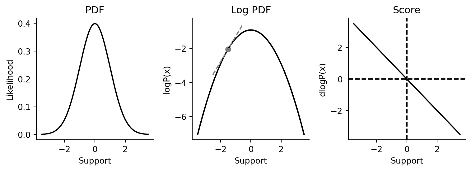
The image below provides a great visual for this. The plot on the left shows a probability density function (our likelihood), and the one in the middle shows its logarithm. Notice how the peak of both curves occurs at the same point on the horizontal axis (in this case, at 0).

A visual comparison of a Gaussian PDF (left), its logarithm (center), and its derivative, the score function (right). For this lesson, observe that the maximum of the PDF and the Log PDF occur at the same value of the support. We will return to the 'Score' plot in a later module.

2. Mathematical and Computational Convenience

Working with sums is far simpler than working with products, especially when it comes to differentiation. To find the maximum of a function, we typically take its derivative, set it to zero, and solve. The derivative of a sum is the sum of the derivatives, a much tidier operation than applying the product rule repeatedly. Furthermore, sums are computationally faster to compute than products.

3. Numerical Stability

This is a critical point for you as a data scientist. Probabilities are numbers between 0 and 1. When you multiply many of these small numbers together, the result can become vanishingly small, leading to a numerical underflow—where the computer's floating-point representation rounds the number down to zero. This would make it impossible to compare the likelihood of different parameter values. Working with the sum of logarithms avoids this entirely, as adding log-probabilities (which are negative numbers) is a much more stable operation.

The following resources provide excellent, concise summaries of these points.

What is log likelihood and why do we use it?

This short video from IntuitiveML gives a very clear and quick summary of the rationale behind using log-likelihood.

Watch the entire video, paying attention to the three key ideas: mathematical simplification, numerical stability, and the monotonicity argument.

Theory and Intuition Behind Numerical MLE

This article provides a well-structured breakdown of the advantages of using the log-likelihood.

Please read the subsection Why Log-Likelihood?. It neatly lists the four main advantages, which we have just discussed.

Log-Likelihood in Action: The Bernoulli Distribution

Let's make this concrete with an example you've likely seen before. We'll find the MLE for the parameter $p$ of a Bernoulli distribution, which models a single coin flip. A Bernoulli random variable $X$ takes the value 1 (heads) with probability $p$ and 0 (tails) with probability $1 - p$ .

The probability mass function (PMF) can be written compactly as:

f (x ∣ p) = p^{x} (1 - p)^{1 - x} for x \in {0, 1}

Given $n$ IID samples $x_{1}, \dots, x_{n}$ , the process of finding the MLE for $p$ using the log-likelihood is a perfect illustration of the principles we've covered.

Maximum Likelihood Estimation

The Stanford course notes we looked at earlier walk through this exact derivation. Following the steps will solidify your understanding of how the log-likelihood simplifies the maximization process.

Start reading from the heading Bernoulli MLE Estimation. Follow the derivation carefully: Likelihood L(p): Note how it's a product. Log-Likelihood \ell(p): See how the log transforms the product into a sum, and exponents become multipliers. Differentiation: Observe how straightforward it is to differentiate the resulting sum with respect to p. Solving for \hat{p}: Setting the derivative to zero yields the intuitive result that the MLE for p is the sample mean.

As you can see, the log-likelihood function not only simplifies the mathematics but also leads to an estimator that is intuitively correct: the best estimate for the probability of heads is the proportion of heads observed in the sample.

Conclusion

In this lesson, we have formally defined the log-likelihood function and established its central role in Maximum Likelihood Estimation. While the concept of MLE may have been familiar, focusing on the "why" behind the logarithm provides a deeper appreciation for the method's elegance and practicality.

The key takeaways are:

The log-likelihood function $ℓ (θ)$ is the natural logarithm of the likelihood function $L (θ)$ .
It transforms the numerically unstable and mathematically difficult product of probabilities into a stable and convenient sum of log-probabilities.
Maximizing the log-likelihood is equivalent to maximizing the likelihood because the logarithm is a strictly monotonic function. This makes it the standard approach for finding Maximum Likelihood Estimates.

In our next lesson, we will build directly on this foundation. We will see how the likelihood function is said to contain all the information in the sample about the unknown parameter. This will lead us to the concept of sufficient statistics and the powerful Neyman-Fisher factorization theorem.

Recommended resources