Spacetime Diagrams: Visualizing Relativity

The Anatomy of a Spacetime Diagram

A spacetime diagram is a graph that visualizes events in spacetime. For simplicity, we'll work with one spatial dimension (x) and time (t).

• Axes: By convention in relativity, the time axis is plotted vertically, and the spatial axis is plotted horizontally. To give both axes the same units of distance, we plot ct on the vertical axis, where c is the speed of light. This choice has a wonderful consequence: the path of a light beam will always have a slope of ±1.
• Events: A single point (x, ct) on the diagram represents an event—something that happens at a specific place and a specific time.
• World Lines: The path of an object as it travels through spacetime is called its world line. It's a curve or line that traces the object's spatial position at every moment in time.

To familiarize yourself with these fundamental concepts, please read the first part of the following resource.

Representing Different Inertial Frames

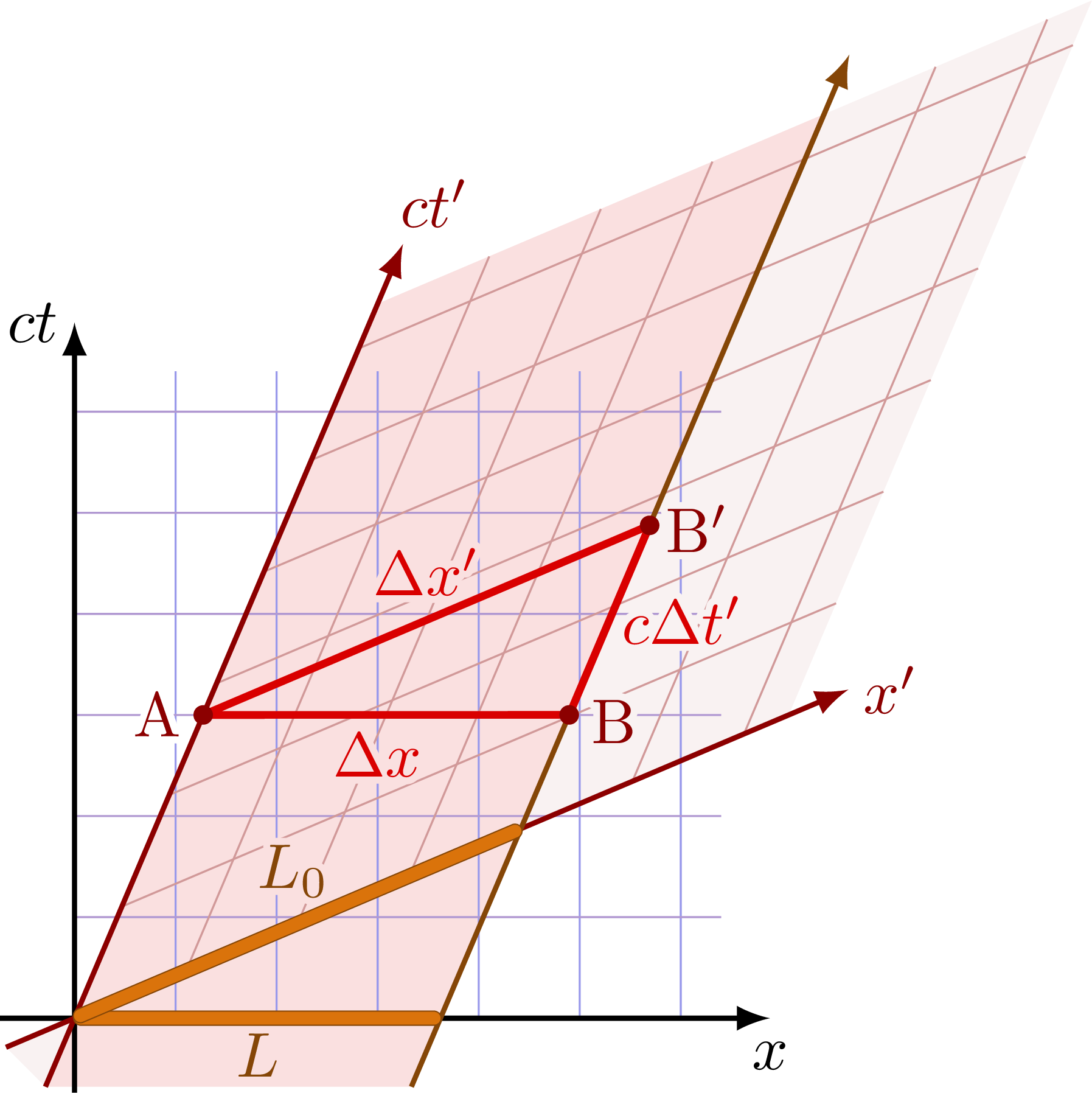
The true power of a Minkowski diagram comes from its ability to represent multiple inertial frames on a single graph. Let's consider our standard two frames: a "stationary" Home Frame S with coordinates (x, t) and an "Other Frame" S' with coordinates (x', t') moving at a velocity v = βc relative to S.

We draw the x and ct axes of frame S as orthogonal (perpendicular) lines. How do we draw the axes of S'?

1. The ct' axis: The time axis of S' represents all events happening at the spatial origin of that frame, i.e., at x' = 0. An object at rest at x' = 0 moves with velocity v in frame S. Its world line in the S frame is given by x = vt. On our diagram, this is a line with a slope of ct/x = c/v = 1/β. This line is the ct' axis.

2. The x' axis: The space axis of S' represents all events that are simultaneous in that frame, i.e., occurring at t' = 0. From our lesson on the relativity of simultaneity, we know that events simultaneous in S' are not simultaneous in S. Using the Lorentz transformation t' = γ(t - vx/c²) = 0, we find that t = (v/c²)x, which corresponds to a line with slope ct/x = v/c = β. This line is the x' axis.

The result is that the axes of the moving frame S' are "scissored" inward relative to the S frame axes. The following video provides an excellent visual derivation of this, starting from first principles.

The Geometry of Spacetime and Visualizing Relativistic Effects

You might be tempted to read coordinates in the S' frame by projecting points perpendicularly onto the skewed axes, as you would in standard Euclidean geometry. This is incorrect. The geometry of spacetime is not Euclidean; it is what we call hyperbolic or Minkowski geometry.

The key to correctly calibrating the axes and reading coordinates lies in the invariance of the spacetime interval. While observers disagree on measurements of space and time separately, they all agree on the value of the quantity $\Delta s^2$, defined as:

$\Delta s^2=(c\Delta t{)}^2-(\Delta x{)}^2$

This is the "distance squared" in Minkowski spacetime. Notice the minus sign, which is the source of all the non-intuitive geometric properties.

In Euclidean space, the set of all points equidistant from the origin forms a circle (x² + y² = R²). In Minkowski spacetime, the set of all points with the same spacetime interval from the origin forms a hyperbola: (ct)² - x² = (Δs)².

These hyperbolas are our calibration curves. A unit of time on the ct' axis is marked where the axis intersects the hyperbola (ct)² - x² = 1. A unit of length on the x' axis is marked where it intersects the hyperbola x² - (ct)² = 1.

With this understanding, we can now visualize time dilation and length contraction.

Time Dilation

Consider an event on the ct' axis, for example, at t' = 1 year. This is the event (x'=0, t'=1). On the diagram, find the t'=1 tick mark on the ct' axis. To find the coordinates of this event in the S frame, we draw lines parallel to the S' axes back to the S axes. A more straightforward way is to read its position relative to the orthogonal S grid. You will see that its ct coordinate is greater than 1. This is time dilation: a single tick of a moving clock corresponds to more than one tick of a stationary clock.

Length Contraction

This is more subtle. Imagine a rod of proper length L_0 at rest in frame S'. Its ends are at x'=0 and x'=L_0. Its world lines are two parallel lines, one being the ct' axis and the other passing through the x'=L_0 tick mark.

To measure its length in frame S, we must find the positions of its two ends at the same time in S. This means we take a horizontal slice across the diagram (a line of constant t). Let's take the slice at t=0, which is the x-axis. The first end of the rod is at the origin (x=0). The second end's world line intersects the x-axis at some value L. As you can see from the geometry, this length L is shorter than L_0. The moving rod is measured to be contracted.

This video walks through how these two effects appear on the diagram.

Causality and the Light Cone

The structure of spacetime imposed by the invariant speed of light has profound implications for cause and effect. From any event (let's place it at the origin), we can draw the world lines of light rays moving outwards. These form a "light cone."

• Future Light Cone: The region of spacetime that can be reached from the origin by traveling at or below the speed of light. Any event caused by the event at the origin must lie in its future light cone.
• Past Light Cone: The region of spacetime from which the origin can be reached. Any event that causes the event at the origin must lie in its past light cone.
• Elsewhere: The region outside the light cone. Events in this region are not causally connected to the event at the origin. A signal would have to travel faster than light to connect them.

The separation between two events can be classified based on the sign of their spacetime interval:

1. Time-like separation ($\Delta s^2>0$): The two events are inside each other's light cones. A massive object can travel between them. Their time-ordering is absolute for all observers (i.e., if event A happens before event B in one frame, it happens before B in all frames).
2. Light-like separation ($\Delta s^2=0$): The events lie on the light cone itself. They can only be connected by a light signal.
3. Space-like separation ($\Delta s^2<0$): The events are outside each other's light cones. They are causally disconnected. The time-ordering of space-like separated events is relative; some observers may see A happen before B, while others see B happen before A.

This next resource provides an excellent, in-depth explanation of these concepts. As someone interested in high-energy physics, the principle of causality is a cornerstone of the theories you will study, like Quantum Field Theory.

Conclusion

Today we've translated the algebra of special relativity into the language of geometry. Spacetime diagrams are not just illustrations; they are analytical tools that provide a deeper, more unified understanding of relativistic physics.

Key Takeaways:

• Spacetime diagrams plot events on a ct vs. x graph, where world lines represent the history of objects.
• An inertial frame moving at velocity v is represented by skewed axes: the ct' axis has a slope of 1/β and the x' axis has a slope of β.
• The geometry of spacetime is not Euclidean. The invariant spacetime interval $\Delta s^2=(c\Delta t{)}^2-(\Delta x{)}^2$ defines the "distance."
• Lines of constant spacetime interval are hyperbolas, which are used to calibrate the axes of moving frames.
• Time dilation and length contraction can be directly visualized on a correctly constructed and calibrated Minkowski diagram.
• The light cone divides spacetime into causally connected (time-like) and disconnected (space-like) regions, defining the structure of cause and effect in the universe.

This lesson concludes our module on the foundations of special relativity. We now have both algebraic (Lorentz transforms) and geometric (Minkowski diagrams) tools at our disposal.

In our next lesson, we will begin the "Relativistic Kinematics" module by formalizing the ideas of spacetime vectors. We will define four-vectors for position, velocity, and momentum. This powerful mathematical framework will allow us to write the laws of physics in a way that is manifestly the same in all inertial frames, a crucial step towards studying relativistic collisions and dynamics.