Fourier Series Representation and Coefficient Calculation

1. The Big Idea: Building Functions from Waves

Imagine you have a complex musical sound. We know that this sound can be broken down into a fundamental frequency and a series of overtones, or harmonics. A Fourier series applies this same idea to mathematical functions.

Any "well-behaved" periodic function $f(x)$ with a period $2L$ can be written as an infinite sum of sines and cosines:

Let's break down this formula:

• $\frac{a_0}{2}$: This is the DC offset or the average value of the function over one period. The factor of 1/2 is a convention that simplifies the general formula for the coefficients.
• The $\sum$: This is the sum of all the harmonics.
• $n=1$ term: This is the fundamental frequency, with a period of $2L$.
• $n>1$ terms: These are the harmonics or overtones, with frequencies that are integer multiples of the fundamental.
• $a_n,b_n$: These are the Fourier coefficients. They determine the amplitude of each cosine and sine wave required to reconstruct the original function $f(x)$.

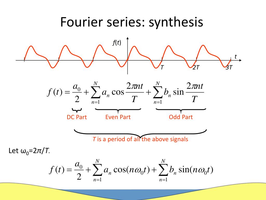
The crucial task is to find a way to calculate these coefficients for any given function $f(x)$.

2. The Key: Orthogonality

To isolate each coefficient, we exploit a remarkable property of sine and cosine functions called orthogonality. In linear algebra, two vectors are orthogonal if their dot product is zero. We can define a similar concept for functions, where the "dot product" is an integral of their product over a specific interval.

For the trigonometric functions in our series, it turns out that the integral of the product of any two different functions over one period ($[-L,L]$) is zero. For example:

This property is what allows us to "filter out" and measure each coefficient one by one.

3. Deriving the Fourier Coefficients (Euler Formulas)

The derivation of the formulas for the coefficients is a beautiful application of these orthogonality relations. Since you appreciate mathematical rigor, the following video provides a complete, step-by-step derivation.

After watching the derivation, the results are a set of three integral formulas, known as the Euler formulas, for the Fourier coefficients of a function $f(x)$ with period $2L$:

The Euler Formulas

(This is twice the average value of the function over one period.)

(This measures the "amount" of $\cos (n\pi x/L)$ in $f(x)$.)

(This measures the "amount" of $\sin (n\pi x/L)$ in $f(x)$.)

These formulas are the core machinery of Fourier analysis. Given any periodic function $f(x)$, you can, in principle, compute its Fourier series representation by evaluating these integrals.

A quick note on convergence: The video briefly mentions the concept of uniform convergence, which is the formal justification for swapping the order of summation and integration in the derivation. For most physically relevant functions (which are piecewise continuous), the Fourier series converges to the function $f(x)$ at all points where $f(x)$ is continuous. At a point of discontinuity (a jump), the series converges to the midpoint of the jump.

4. Simplifications: Even and Odd Functions

Calculating all those integrals can be tedious. However, we can often use symmetry to simplify the work. This is a common strategy in physics.

As you've just read, the key takeaways are:

• Even Functions: If $f(x)$ is even ($f(-x)=f(x)$), its graph is symmetric about the y-axis. Its Fourier series will contain only cosine terms (and possibly the $a_0$ constant term). All $b_n$ coefficients are zero. $$b_n=0,a_n=\frac{2}{L}{\int }_0^{L}f(x)\cos \left(\frac{n\pi x}{L}\right)dx$$
• Odd Functions: If $f(x)$ is odd ($f(-x)=-f(x)$), its graph has rotational symmetry about the origin. Its Fourier series will contain only sine terms. All $a_n$ coefficients (including $a_0$) are zero. $$a_n=0,b_n=\frac{2}{L}{\int }_0^{L}f(x)\sin \left(\frac{n\pi x}{L}\right)dx$$

Recognizing the symmetry of a function before you start integrating can save you half the work!

An Application: The Square Wave and Gibbs Phenomenon

Let's apply this to a classic example: a square wave. Consider an even square wave with period $2L=2\pi$ ($L=\pi$) defined as:
$f(x)=\{\begin{array}{ll}1& \text{if }-\pi /2<x<\pi /2\\ -1& \text{if }\pi /2<x<3\pi /2\end{array}$
Since this is an even function, we know $b_n=0$. We only need to calculate $a_n$.
$a_0=\frac{1}{\pi }{\int }_{-\pi }^{\pi }f(x)dx=\frac{1}{\pi }\left({\int }_{-\pi /2}^{\pi /2}1dx+{\int }_{\pi /2}^{3\pi /2}(-1)dx\right)=\frac{1}{\pi }(\pi -\pi )=0$.

Using the simplified formula for even functions:
$a_n=\frac{2}{\pi }{\int }_0^{\pi }f(x)\cos (nx)dx=\frac{2}{\pi }\left({\int }_0^{\pi /2}1\cdot \cos (nx)dx+{\int }_{\pi /2}^{\pi }(-1)\cdot \cos (nx)dx\right)$
$a_n=\frac{2}{\pi }\left({\left[\frac{\sin (nx)}{n}\right]}_0^{\pi /2}-{\left[\frac{\sin (nx)}{n}\right]}_{\pi /2}^{\pi }\right)=\frac{2}{n\pi }(\sin (n\pi /2)-0-(\sin (n\pi )-\sin (n\pi /2)))$
$a_n=\frac{4}{n\pi }\sin \left(\frac{n\pi }{2}\right)$
This results in $a_n=0$ for even $n$, and alternating values for odd $n$. The final series is:
$f(x)=\frac{4}{\pi }\left(\cos (x)-\frac{1}{3}\cos (3x)+\frac{1}{5}\cos (5x)-\cdots \right)$
If we plot the partial sums of this series, we see it approximates the square wave, but with a peculiar overshoot at the discontinuities. This is called the Gibbs phenomenon.

Conclusion

Today we've unlocked a method for deconstructing complex periodic functions into simple, manageable building blocks. This is a cornerstone of mathematical physics.

Key Takeaways:

• A periodic function $f(x)$ with period $2L$ can be represented by a Fourier series, an infinite sum of cosine and sine terms.
• The coefficients $a_n$ and $b_n$ are determined by the Euler formulas, which are derived using the orthogonality of sine and cosine functions over the interval $[-L,L]$.
• If a function is even, its Fourier series contains only cosine terms. If it is odd, it contains only sine terms. This symmetry can significantly simplify calculations.
• The Fourier series approximation of a function with a jump discontinuity exhibits an overshoot known as the Gibbs phenomenon.

Preview of the Next Lesson:
We've spent the last two lessons focused on functions of a single variable (often time). Now, we will shift our focus to functions декораof multiple spatial variables, known as fields. In the next lesson, we will begin our study of vector calculus by defining three fundamental differential operators: the gradient, divergence, and curl. These operators are the language of field theories like electromagnetism and fluid dynamics, and they will be essential tools for the rest of our journey.