Electrostatic Field: Conservative Nature and Electric Potential

1. Work, Path Independence, and Conservative Fields

Let's start with a physical concept you're familiar with from mechanics: work. The work done by an electric field $\mathbf{E}$ on a unit positive charge moving along a path $C$ from point A to point B is given by the line integral:
$W_{A\to B}={\int }_A^B\mathbf{E}\cdot d\mathbf{l}$
A key question is: does the amount of work done depend on the specific path taken between A and B? For the electrostatic field, the answer is no. This makes it a conservative field.

This path independence is a direct consequence of the $1/r^2$ nature of Coulomb's law. We can prove this mathematically for the field of a single point charge, and then, using the principle of superposition, extend it to any electrostatic field produced by a static distribution of charges.

A crucial consequence of path independence is that the work done around any closed loop is zero. If you start at point A and return to point A, the net work done by the field is zero, regardless of the path you take.
$\oint \mathbf{E}\cdot d\mathbf{l}=0$
This is the integral form of the statement that the electrostatic field is conservative.

2. The Curl of the Electric Field

We've established the integral property of a conservative field. Now, let's find its equivalent differential form. This requires introducing a new vector operator: the curl, denoted $\nabla \times$.

Physically, the curl of a vector field at a point measures the "circulation" or "rotation" of the field in the infinitesimal neighborhood of that point. Imagine placing a tiny paddle wheel in a fluid flow; if the wheel spins, the velocity field has a non-zero curl.

The mathematical bridge between the closed-loop integral and the curl is Stokes' Theorem:
${\oint }_C\mathbf{F}\cdot d\mathbf{l}={\iint }_S(\nabla \times \mathbf{F})\cdot d\mathbf{S}$
This theorem states that the line integral of a vector field $\mathbf{F}$ around a closed curve $C$ is equal to the flux of its curl through any surface $S$ bounded by that curve.

Now, let's apply this to the electrostatic field $\mathbf{E}$. We already know from Section 1 that $\oint \mathbf{E}\cdot d\mathbf{l}=0$ for any closed loop. According to Stokes' Theorem, this means:
${\iint }_S(\nabla \times \mathbf{E})\cdot d\mathbf{S}=0$
Since this must hold for any surface $S$, the integrand itself must be zero everywhere. This leads us to our second fundamental equation of electrostatics:
$\nabla \times \mathbf{E}=0$

This equation is the differential statement that the electrostatic field is conservative. It's the second of Maxwell's equations in its static form.

3. Defining the Electric Potential

The fact that the work done is path-independent allows us to define a scalar field called the electric potential, denoted $\varphi$ or $V$. This is analogous to how gravitational potential energy can be defined because the gravitational force is also conservative.

The potential difference between two points B and A is defined as the work done per unit charge in moving a charge from A to B against the electric field.
$\Delta V=V_B-V_A=-{\int }_A^B\mathbf{E}\cdot d\mathbf{l}$
The minus sign is a crucial convention: it ensures that positive charges, when free to move, will travel from a region of higher potential to a region of lower potential, just as a ball rolls downhill. The unit of potential is the Volt (V), where 1 Volt = 1 Joule/Coulomb.

To define an absolute potential at a single point, we must choose a reference point where the potential is set to zero. By convention in electromagnetism, this reference point is usually taken to be at infinity. The potential at a point P is then the work per unit charge to bring a charge from infinity to P:
$V(P)=-{\int }_{\infty }^P\mathbf{E}\cdot d\mathbf{l}$

For a point charge $q$ at the origin, we can calculate its potential at a distance $r$:
$V(r)=-{\int }_{\infty }^r\frac{q}{4\pi {ϵ}_0{r}^{\prime 2}}\hat{\mathbf{r}}\cdot d\mathbf{l}=-{\int }_{\infty }^r\frac{q}{4\pi {ϵ}_0{r}^{\prime 2}}d{r}^{\prime }={\left[\frac{q}{4\pi {ϵ}_0{r}^{\prime }}\right]}_{\infty }^r=\frac{q}{4\pi {ϵ}_{0}r}$
One of the great advantages of potential is that it is a scalar. To find the total potential from a collection of charges, you simply add the potentials from each charge—a simple scalar sum, much easier than the vector sum required for electric fields.

4. Recovering the Field from the Potential

We've defined potential by integrating the electric field. Can we go the other way? Yes. The relationship between field and potential is fundamental.

From the definition of potential difference, an infinitesimal change in potential $dV$ when moving by a displacement $d\mathbf{l}$ is:
$dV=-\mathbf{E}\cdot d\mathbf{l}$
From multivariable calculus, we also know that the total differential of a scalar function $V(x,y,z)$ is:
$dV=\frac{\partial V}{\partial x}dx+\frac{\partial V}{\partial y}dy+\frac{\partial V}{\partial z}dz$
This can be written as the dot product of the gradient of V and the displacement vector $d\mathbf{l}$:
$dV=(\nabla V)\cdot d\mathbf{l}$
Comparing our two expressions for $dV$, we find the crucial relationship:
$\mathbf{E}=-\nabla V$
The electric field is the negative gradient of the electric potential. This powerful result means that if you can find the scalar potential $V$ (which is often easy), you can calculate the vector electric field $\mathbf{E}$ by taking its gradient.

The physical meaning is clear: the gradient $\nabla V$ points in the direction of the steepest increase in potential. The negative sign tells us that the electric field $\mathbf{E}$ points in the direction of the steepest decrease in potential—"downhill". This also implies that electric field lines are always perpendicular to surfaces of constant potential (equipotential surfaces).

5. Application: High-Level Problem Solving

Your goal includes tackling competitive-level problems. Problems involving potential are very common because scalar calculations are often simpler than vector ones, especially in symmetric configurations.

Let's analyze a problem from the JEE Advanced exam.

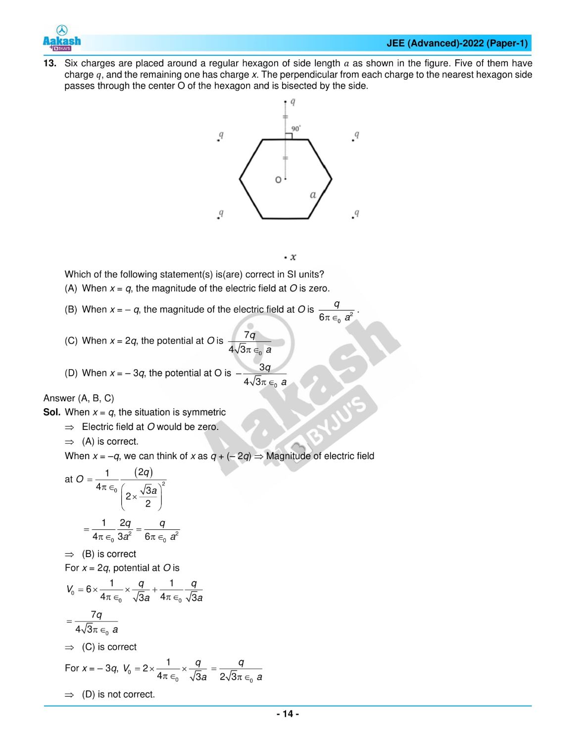
Let's analyze this using the concepts from this lesson:

1. Potential (V):

   • The potential at the center O is the scalar sum of the potentials from each of the six charges.
   • Each vertex is at the same distance 'a' from the center.
   • The potential from a single charge $q_i$ at distance 'a' is $V_i=q_i/(4\pi {ϵ}_{0}a)$.
   • Total potential: $V_{total}=\frac{1}{4\pi {ϵ}_{0}a}\sum q_i=\frac{1}{4\pi {ϵ}_{0}a}(5q+x)$.
   • If $x=q$, then $V=\frac{6q}{4\pi {ϵ}_{0}a}$.
   • If $x=-q$, then $V=\frac{4q}{4\pi {ϵ}_{0}a}$.

2. Electric Field (E):

   • The electric field is a vector sum.
   • If $x=q$, all six charges are identical. By symmetry, the vector sum of the fields from the six charges at the center is zero. The field from any charge is exactly cancelled by the field from the charge directly opposite it.
   • If $x=-q$, imagine this as a full hexagon of +q charges (where E=0) plus a superposition of a -2q charge at the position of x (since $q+(-2q)=-q$). The field from the full hexagon of +q is zero, so the total field is just the field from a single -2q charge. Its magnitude would be $E=\frac{2q}{4\pi {ϵ}_0{a}^2}$.

This problem demonstrates the power of using both potential (for its scalar simplicity) and field (leveraging vector symmetry) to analyze a system.

Conclusion

This lesson has been pivotal. We have established one of the most fundamental properties of the electrostatic field and introduced its most useful mathematical tool.

Key Takeaways:

• Conservative Field: The electrostatic field is conservative, meaning the work done moving a charge between two points is path-independent.
• Integral and Differential Forms: This property is expressed in integral form as $\oint \mathbf{E}\cdot d\mathbf{l}=0$ and in differential form as $\nabla \times \mathbf{E}=0$. This is the second of Maxwell's equations for electrostatics.
• Electric Potential: The conservative nature of $\mathbf{E}$ allows us to define a scalar electric potential $V$, where the potential difference is $V_B-V_A=-{\int }_A^B\mathbf{E}\cdot d\mathbf{l}$.
• Field from Potential: The electric field can be recovered from the potential using the relation $\mathbf{E}=-\nabla V$. This often simplifies problems enormously, reducing a vector problem to a scalar one.

Preview of the Next Lesson:
We now have two of Maxwell's equations for electrostatics: $\nabla \cdot \mathbf{E}=\rho /{ϵ}_0$ and $\nabla \times \mathbf{E}=0$. By combining these with $\mathbf{E}=-\nabla V$, we can derive a powerful second-order differential equation for the potential itself, known as Poisson's Equation (${\nabla }^{2}V=-\rho /{ϵ}_0$) and its special case, Laplace's Equation. In the next lesson, we will derive these equations and begin exploring the powerful techniques used to solve them in boundary-value problems.