Magnetic Vector Potential and Field Derivations

1. Defining the Magnetic Vector Potential, $\mathbf{A}$

In electrostatics, the fact that the electrostatic field is conservative ($\nabla \times \mathbf{E}=0$) allowed us to define a scalar potential $\varphi$ such that $\mathbf{E}=-\nabla \varphi$. We are going to use a similar line of reasoning for the magnetic field.

One of the fundamental equations of magnetostatics (and one of Maxwell's equations) states that the magnetic field is always divergenceless:
$\nabla \cdot \mathbf{B}=0$
This is the mathematical expression of the experimental fact that there are no magnetic monopoles.

Now, recall the vector calculus identity that the divergence of the curl of any vector field is always zero:
$\nabla \cdot (\nabla \times \mathbf{F})=0\text{for any vector field }\mathbf{F}$
Comparing these two equations, we see that since $\nabla \cdot \mathbf{B}=0$, it is mathematically guaranteed that we can express $\mathbf{B}$ as the curl of some other vector field. We call this field the magnetic vector potential, $\mathbf{A}$.

Definition: Magnetic Vector Potential
$\mathbf{B}=\nabla \times \mathbf{A}$

This definition is the cornerstone of our new method. To find $\mathbf{B}$, we can now try to find $\mathbf{A}$ first and then take its curl. The following video provides a concise explanation of this crucial first step.

2. Relating the Vector Potential to the Current Density

We have defined $\mathbf{A}$, but how do we find it from a given distribution of currents? Our goal is to derive an equation that relates $\mathbf{A}$ to the current density $\mathbf{J}$.

We start with the differential form of Ampère's Law, which you learned in the previous lesson:
$\nabla \times \mathbf{B}={\mu }_0\mathbf{J}$
Now, substitute our new definition, $\mathbf{B}=\nabla \times \mathbf{A}$:
$\nabla \times (\nabla \times \mathbf{A})={\mu }_0\mathbf{J}$
This expression can be simplified using the vector identity $\nabla \times (\nabla \times \mathbf{F})=\nabla (\nabla \cdot \mathbf{F})-{\nabla }^2\mathbf{F}$. Applying this to $\mathbf{A}$, we get:
$\nabla (\nabla \cdot \mathbf{A})-{\nabla }^2\mathbf{A}={\mu }_0\mathbf{J}$
This equation looks more complicated than what we started with. However, we have a degree of freedom we can use to simplify it.

Gauge Freedom and the Coulomb Gauge

The definition $\mathbf{B}=\nabla \times \mathbf{A}$ does not uniquely define $\mathbf{A}$. If we take a new potential ${\mathbf{A}}^{\prime }=\mathbf{A}+\nabla \chi$, where $\chi$ is any scalar function, the magnetic field remains unchanged because $\nabla \times (\nabla \chi )=0$. This freedom to change the potential without changing the physical field is known as a gauge transformation.

We can exploit this freedom to impose an extra condition on $\mathbf{A}$ to simplify our equation. In magnetostatics, the most convenient choice is the Coulomb gauge (also called the transverse gauge):
$\nabla \cdot \mathbf{A}=0$
By choosing this gauge, the $\nabla (\nabla \cdot \mathbf{A})$ term in our equation vanishes, leaving us with a much simpler result.

The Poisson Equation for $\mathbf{A}$

With the Coulomb gauge condition, our equation becomes:
${\nabla }^2\mathbf{A}=-{\mu }_0\mathbf{J}$
This is the vector Poisson equation. It's a set of three separate Poisson equations, one for each Cartesian component of $\mathbf{A}$:
${\nabla }^2{A}_x=-{\mu }_0{J}_x,{\nabla }^2{A}_y=-{\mu }_0{J}_y,{\nabla }^2{A}_z=-{\mu }_0{J}_z$
You will recognize that this is directly analogous to the Poisson equation for the electric potential, ${\nabla }^2\varphi =-\rho /{ϵ}_0$. The solution is also analogous. Just as the solution for $\varphi$ is $\varphi (\mathbf{r})=\frac{1}{4\pi {ϵ}_0}\int \frac{\rho ({\mathbf{r}}^{\prime })}{|\mathbf{r}-{\mathbf{r}}^{\prime }|}{d}^3{r}^{\prime }$, the solution for $\mathbf{A}$ is:

Integral Solution for the Vector Potential
$\mathbf{A}(\mathbf{r})=\frac{{\mu }_0}{4\pi }\int \frac{\mathbf{J}({\mathbf{r}}^{\prime })}{|\mathbf{r}-{\mathbf{r}}^{\prime }|}{d}^3{r}^{\prime }$

This integral is our primary tool for calculating the vector potential from a known current distribution.

The following video walks through this derivation, providing a clear explanation of each step.

3. Application: Finding the Magnetic Field

Now we have a complete procedure:

1. For a given current distribution $\mathbf{J}$, calculate the vector potential $\mathbf{A}$ using the integral solution.
2. Calculate the magnetic field $\mathbf{B}$ by taking the curl of the potential: $\mathbf{B}=\nabla \times \mathbf{A}$.

While this two-step process might seem longer, the integral for $\mathbf{A}$ is often much easier to solve than the vector integral in the Biot-Savart law.

Example: Finite Straight Wire

Let's apply this method to a problem that is non-trivial with the Biot-Savart law: finding the field of a finite straight wire of length $a$. The following video provides a rigorous and detailed walkthrough of both steps: calculating $\mathbf{A}$ and then taking its curl to find $\mathbf{B}$. This is a substantial calculus exercise, exactly the kind of rigorous problem you appreciate.

This example shows that even when the calculus is demanding, this method provides a systematic path to the solution. The advantage is that we deal with a vector potential integral first (which can be easier), and then perform a local differentiation (the curl).

Test your understanding!

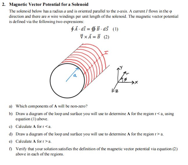
For a highly symmetric system like an ideal (infinite) solenoid, there's a shortcut to find $\mathbf{A}$ that avoids direct integration over the current distribution. We can use Stokes' Theorem on the definition of $\mathbf{A}$:
${\oint }_C\mathbf{A}\cdot d\mathbf{l}={\int }_S(\nabla \times \mathbf{A})\cdot d\mathbf{S}={\int }_S\mathbf{B}\cdot d\mathbf{S}={\Phi }_B$
This says the circulation of $\mathbf{A}$ around a closed loop is equal to the magnetic flux ${\Phi }_B$ through the surface bounded by that loop.

Use this principle and the problem statement in the image below to find the vector potential $\mathbf{A}$ both inside ($r<a$) and outside ($r>a$) a long solenoid.

Show answer

From the last lesson, we know the field inside an ideal solenoid is $\mathbf{B}={\mu }_{0}nI\hat{\mathbf{z}}$ and outside is $\mathbf{B}=0$. Due to the cylindrical symmetry and the current flowing in the $\hat{\mathbf{\varphi }}$ direction, we assume $\mathbf{A}$ has the form $\mathbf{A}=A(r)\hat{\mathbf{\varphi }}$.

We choose a circular Amperian loop of radius $r$ concentric with the solenoid's axis. The left side of the equation becomes:
${\oint }_C\mathbf{A}\cdot d\mathbf{l}={\int }_0^{2\pi }A(r)\hat{\mathbf{\varphi }}\cdot (rd\varphi \hat{\mathbf{\varphi }})=A(r)\cdot 2\pi r$

1. Inside the solenoid ($r<a$):
The magnetic flux through the circular loop is ${\Phi }_B=\int \mathbf{B}\cdot d\mathbf{S}=({\mu }_{0}nI)\cdot (\pi r^2)$.
Equating the two sides:
$A(r)\cdot 2\pi r={\mu }_{0}nI\pi r^2⟹A(r)=\frac{{\mu }_{0}nIr}{2}$
So, inside the solenoid, $\mathbf{A}=\frac{{\mu }_{0}nIr}{2}\hat{\mathbf{\varphi }}$.

2. Outside the solenoid ($r>a$):
The magnetic field is non-zero only within the radius $a$. So the flux through our loop of radius $r>a$ is confined to the solenoid's cross-section: ${\Phi }_B=({\mu }_{0}nI)\cdot (\pi a^2)$.
Equating the two sides:
$A(r)\cdot 2\pi r={\mu }_{0}nI\pi a^2⟹A(r)=\frac{{\mu }_{0}nI{a}^2}{2r}$
So, outside the solenoid, $\mathbf{A}=\frac{{\mu }_{0}nI{a}^2}{2r}\hat{\mathbf{\varphi }}$.

You can verify that taking the curl of these expressions for $\mathbf{A}$ correctly reproduces the known magnetic field $\mathbf{B}$.

Advanced Problem: Infinite Current Sheet

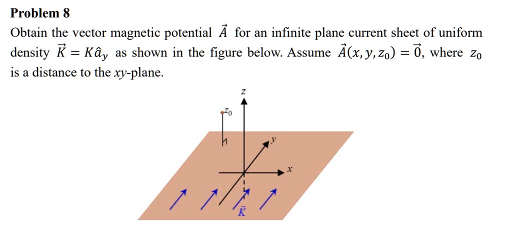
Consider an infinite sheet of current in the $xy$-plane with uniform surface current density $\mathbf{K}=K\hat{\mathbf{y}}$. In terms of 3D current density, this is $\mathbf{J}=K\delta (z)\hat{\mathbf{y}}$.

Your task is to find the vector potential $\mathbf{A}$.

Hint: Start with the Poisson equation ${\nabla }^2\mathbf{A}=-{\mu }_0\mathbf{J}$. Given the symmetries, what form must $\mathbf{A}$ take? The problem simplifies to a 1D differential equation.

Show answer

1. Symmetry: Since the current $\mathbf{J}$ is only in the $\hat{\mathbf{y}}$ direction, the vector potential $\mathbf{A}$ will also only have a $\hat{\mathbf{y}}$ component. Furthermore, since the sheet is infinite in $x$ and $y$, the potential can only depend on $z$. So, we look for a solution of the form $\mathbf{A}(z)=A_y(z)\hat{\mathbf{y}}$.

2. Poisson's Equation: The vector Poisson equation ${\nabla }^2\mathbf{A}=-{\mu }_0\mathbf{J}$ simplifies to a single 1D equation:
   $\frac{d^2{A}_y}{d{z}^2}=-{\mu }_{0}K\delta (z)$

3. Solving the Equation: We can solve this by integrating twice. Integrating once gives the derivative:
   $\frac{d{A}_y}{dz}=-{\mu }_{0}K\int \delta (z)dz=-{\mu }_{0}K\cdot H(z)+C_1$
   where $H(z)$ is the Heaviside step function. By symmetry ($B_x(z)=-B_x(-z)$, and $B_x=-d{A}_y/dz$), we must have the derivative be an odd function of $z$, which sets $C_1={\mu }_{0}K/2$. So, $\frac{d{A}_y}{dz}=-\frac{{\mu }_{0}K}{2}\text{sgn}(z)$. This correctly gives the magnetic field $\mathbf{B}=\nabla \times \mathbf{A}=(\frac{d{A}_y}{dz})\hat{\mathbf{x}}=-\frac{{\mu }_{0}K}{2}\text{sgn}(z)\hat{\mathbf{x}}$, which matches the result from Ampère's Law.

4. Integrating Again: Integrating $\frac{d{A}_y}{dz}$ gives $A_y(z)$:
   $A_y(z)=-\frac{{\mu }_{0}K}{2}\int \text{sgn}(z)dz=-\frac{{\mu }_{0}K}{2}|z|+C_2$
   We can set the integration constant $C_2=0$ by choosing our potential to be zero at $z=0$.

5. Final Result: The vector potential is:
   $\mathbf{A}(z)=-\frac{{\mu }_{0}K}{2}|z|\hat{\mathbf{y}}$

Conclusion

In this lesson, we have developed a powerful and general framework for solving magnetostatics problems. By introducing the magnetic vector potential, we've created a method that is often more tractable than the Biot-Savart law and not limited by the high symmetry required by Ampère's law.

Key Takeaways:

• The condition $\nabla \cdot \mathbf{B}=0$ guarantees that the magnetic field can be written as the curl of a vector potential: $\mathbf{B}=\nabla \times \mathbf{A}$.
• Using the Coulomb gauge ($\nabla \cdot \mathbf{A}=0$), the vector potential is related to the current density by the vector Poisson equation: ${\nabla }^2\mathbf{A}=-{\mu }_0\mathbf{J}$.
• The general integral solution for the vector potential is $\mathbf{A}(\mathbf{r})=\frac{{\mu }_0}{4\pi }\int \frac{\mathbf{J}({\mathbf{r}}^{\prime })}{|\mathbf{r}-{\mathbf{r}}^{\prime }|}{d}^3{r}^{\prime }$.
• The standard workflow is to first calculate $\mathbf{A}$ (either by integration or by solving the differential equation) and then find the magnetic field via $\mathbf{B}=\nabla \times \mathbf{A}$.

Preview of the Next Lesson:
So far, we have focused on calculating the static fields produced by steady currents. But what happens when we place a moving charge in an existing electric and magnetic field? In the next lesson, we will study the Lorentz force, which describes the total force on a charged particle in combined $\mathbf{E}$ and $\mathbf{B}$ fields. This will allow us to analyze the trajectory of particles in various field configurations, a topic with direct applications in areas like particle accelerators and mass spectrometry. We will also see that the vector potential $\mathbf{A}$ is not just a mathematical convenience; it plays a profound role in the advanced Lagrangian and Hamiltonian formulations of classical and quantum mechanics, which is a key step on your path toward theoretical physics.