Gradient Descent vs. Normal Equation: A Trade-off Analysis

Hello! Welcome to the next lesson in our journey through supervised learning.

In the last lesson, you successfully implemented the Normal Equation, a remarkably direct method for finding the optimal parameters for linear regression in a single step. This likely raised an important question: if we have this powerful, one-shot formula, why did we spend so much time implementing and tuning the iterative gradient descent algorithm?

Today, we will answer that question directly. Our goal is to compare the computational and practical trade-offs between gradient descent and the normal equation. By the end of this lesson, you'll have a clear framework for deciding which optimization method is the right tool for a given job.

1. The Destination vs. The Journey

For a standard linear regression problem, both Gradient Descent and the Normal Equation aim to find the parameters that minimize the Mean Squared Error. In most cases, they will arrive at virtually identical solutions.

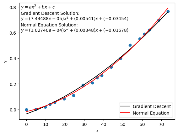
Comparison of Gradient Descent and Normal Equation Solutions for Quadratic Regression — This plot shows that for a given dataset, the curves fitted by Gradient Descent and the Normal Equation are nearly indistinguishable. The difference lies not in the final result, but in how they get there.

The choice between them is not about which one is "more correct," but about which one is more efficient and practical for a specific scenario. Let's break down the key differences.

2. A Head-to-Head Comparison

We can analyze the trade-offs across several key dimensions: the underlying approach, computational cost, and practical requirements.

Approach: Iterative vs. Analytical

This is the most fundamental difference.

Gradient Descent (GD) is an iterative algorithm. It starts with an initial guess for the parameters ( $θ$ ) and takes many small steps "downhill" on the cost function landscape until it converges to a minimum. This process is guided by a learning rate ( $α$ ) that you have to choose and tune.
The Normal Equation (NE) is an analytical solution. It solves for the optimal $θ$ directly using a mathematical formula: $θ = (X^{T} X)^{- 1} X^{T} y$ . There are no iterations, no initial guesses, and no hyperparameters like a learning rate to tune.

This distinction is summarized well in the following article.

Normal Equation for Linear Regression Tutorial

The article 'Normal Equation for Linear Regression Tutorial' from DataCamp provides a concise overview of the differences. Focus on the section comparing the two methods.

Read the section titled 'The Normal Equation vs Gradient Descent'. Pay attention to how it contrasts the iterative nature of GD with the direct, analytical approach of the Normal Equation, and the implications for the learning rate.

Computational Complexity: The Deciding Factor

Given your background in computer science, the analysis of algorithmic complexity will be the most insightful part of this comparison. The choice between GD and NE often boils down to the number of features in your dataset.

Normal Equation: The computational bottleneck is inverting the X.T @ X matrix. This matrix has dimensions of $(n + 1) \times (n + 1)$ , where $n$ is the number of features. The time complexity of inverting a matrix is approximately $O (n^{3})$ . This is manageable for a small number of features, but it becomes extremely slow as $n$ grows. If you have 100,000 features, n^3 is a prohibitively large number.
Gradient Descent: The complexity of one iteration of batch gradient descent is roughly $O (m \cdot n)$ , where $m$ is the number of training samples. The total cost is $O (k \cdot m \cdot n)$ , where $k$ is the number of iterations.

The key insight is that the cost of GD scales linearly with the number of features, whereas the cost of NE scales cubically.

Normal Equation for Linear Regression Tutorial

The same DataCamp article explains this critical trade-off.

Now, read the section 'Deciphering When to Use the Normal Equation'. This part explicitly discusses the O(n^3) complexity and provides a practical rule of thumb from Andrew Ng regarding the number of features.

As the article mentions, a common heuristic is:

If n < 10,000, the Normal Equation is often faster and simpler.
If n > 10,000, Gradient Descent is the necessary choice to avoid the crippling $O (n^{3})$ cost.

Practical Considerations

Beyond pure computational speed, there are other practical differences:

Feature Scaling: As you saw when implementing it, Gradient Descent's convergence speed is highly dependent on feature scaling. The Normal Equation does not require feature scaling at all, which removes a data preprocessing step.
Flexibility: This is a major point. The Normal Equation is only applicable to Linear Regression (specifically, models where the cost function is a simple quadratic). Gradient Descent, on the other hand, is a general-purpose optimization algorithm. You will reuse and adapt your GD implementation for many other models in this course, including Logistic Regression, SVMs, and Neural Networks. Learning GD is an investment that pays off for the rest of your machine learning journey.

Test your understanding!

Imagine you are building a model to predict house prices. In scenario A, you have 5 features (size, bedrooms, age, distance to city center, school rating) and 1 million house listings. In scenario B, you are working on a bioinformatics problem with 500 patient samples but 20,000 features per sample (gene expression levels).

Which optimization algorithm would you choose for each scenario and why?

Show answer

Scenario A (m=1,000,000, n=5): The Normal Equation is the better choice. The number of features n is very small (5), so calculating the inverse of a 6x6 matrix is trivial ((5+1)x(5+1)). The cost, O(n^3), will be negligible. While Gradient Descent would also work, the Normal Equation is simpler as it requires no hyperparameter tuning. Even with a large m, the matrix multiplications in the Normal Equation are computationally feasible.
Scenario B (m=500, n=20,000): Gradient Descent is the only feasible option. The number of features n is very large (20,000). Trying to invert a 20,001 x 20,001 matrix would be computationally impossible for most systems due to the O(n^3) complexity. Gradient Descent's complexity O(k*m*n) scales much more gracefully with the number of features.

3. Summary Table

Let's consolidate these differences into a clear table. The following resource provides a perfect summary.

Difference between Gradient descent and Normal equation

The article 'Difference between Gradient descent and Normal equation' from GeeksforGeeks contains an excellent summary table.

Study the table in the section 'Difference between Gradient Descent and the Normal Equation.' It provides a side-by-side comparison of the key features we've discussed.

Here is a summary of that information for quick reference:

Feature	Gradient Descent	Normal Equation
Approach	Iterative	Analytical (closed-form solution)
Hyperparameters	Needs learning rate ( $α$ ), iterations	None
Feature Scaling	Required for good performance	Not required
Complexity	$O (k \cdot m \cdot n)$	$O (n^{3})$
Best for...	Large number of features ( $n$ )	Small number of features ( $n$ )
Applicability	General purpose (Linear/Logistic Reg, NN, etc.)	Linear Regression only
Implementation	Requires a loop and update rule	A single formula, often one line in NumPy

Conclusion

You now have a solid understanding of the trade-offs between two fundamental optimization approaches. The Normal Equation is a highly efficient, specialized tool, while Gradient Descent is the versatile, scalable workhorse of machine learning.

Key Takeaways:

The primary factor when choosing between Gradient Descent and the Normal Equation is the number of features ( $n$ ).
Normal Equation is preferred for small $n$ (e.g., < 10,000) due to its $O (n^{3})$ complexity and lack of hyperparameters.
Gradient Descent is necessary for large $n$ and is a far more versatile algorithm that you will use to train most other models in machine learning.
The choice is about computational efficiency and practicality, not about which method produces a "better" result for linear regression.

Preview of the Next Lesson:
We are now ready to move from regression problems (predicting continuous values) to classification problems (predicting discrete categories). In the next module, we will start building our first classifier: Logistic Regression. You'll see immediately why our deep dive into Gradient Descent was so important, as we'll use it to optimize a brand new type of cost function. Our first step will be to implement the core component of logistic regression: the sigmoid function.

Recommended resources