Finding the Best Split in a Dataset

The Search for the Best Split

We know that a "good" split is one that maximizes information gain. But how do we find the best one out of all possibilities? The approach, often called a greedy search, is straightforward yet powerful:

1. Initialize a variable best_gain to a very low value (e.g., -1).
2. Create a nested loop:
   • The outer loop iterates through every feature (column) in our dataset X.
   • The inner loop iterates through every unique value within that feature. Each unique value is a potential threshold for a split.
3. Inside the inner loop, for each (feature, threshold) pair:
   • Split the dataset into a left node (where feature <= threshold) and a right node (where feature > threshold).
   • Calculate the information gain for this split using the information_gain function you built in the previous lesson.
   • If this calculated gain is greater than best_gain, update best_gain with the new value and store the current feature and threshold as the best ones found so far.
4. After checking all features and all their unique values, the function will return the feature and threshold that produced the highest information gain.

This process ensures we've exhaustively checked every possible way to split the data at a given node and selected the most informative one.

To see this logic explained with a code walkthrough, let's watch a segment from a helpful video.

Implementing the Best Split Function

Now, let's implement this from scratch. We'll break it down into two parts: a small helper function to perform the split, and the main function that searches for the best split.

1. A Helper Function to Split the Data

First, we need a simple function that takes a dataset (X and y), a feature index, and a threshold, and divides the data into two subsets. Your proficiency with NumPy's boolean indexing will make this straightforward.

import numpy as np
from collections import Counter

# --- Assume these functions from the previous lesson are available ---
def gini_impurity(y):
    counts = Counter(y)
    if len(counts) <= 1: return 0
    impurity = 1.0
    num_samples = len(y)
    for label in counts:
        prob_of_label = counts[label] / num_samples
        impurity -= prob_of_label**2
    return impurity

def information_gain(parent_y, left_y, right_y):
    if len(left_y) == 0 or len(right_y) == 0: return 0
    parent_impurity = gini_impurity(parent_y)
    n_parent = len(parent_y)
    n_left, n_right = len(left_y), len(right_y)
    weight_left = n_left / n_parent
    weight_right = n_right / n_parent
    weighted_child_impurity = (weight_left * gini_impurity(left_y) + 
                               weight_right * gini_impurity(right_y))
    ig = parent_impurity - weighted_child_impurity
    return ig
# --------------------------------------------------------------------

def split_dataset(X, y, feature_index, threshold):
    """
    Splits a dataset based on a feature and a threshold.
    
    Args:
        X (np.ndarray): The feature matrix.
        y (np.ndarray): The target vector.
        feature_index (int): The index of the feature to split on.
        threshold (float): The threshold value for the split.
        
    Returns:
        A tuple of (X_left, y_left, X_right, y_right).
    """
    # Create a boolean mask for the left split (feature <= threshold)
    left_mask = X[:, feature_index] <= threshold
    
    # The right split is the inverse of the left mask
    right_mask = ~left_mask
    
    # Apply the masks to get the subsets
    X_left, y_left = X[left_mask], y[left_mask]
    X_right, y_right = X[right_mask], y[right_mask]
    
    return X_left, y_left, X_right, y_right

This function is our basic data partitioning tool. Now we can use it inside our main search function.

2. The find_best_split Function

This is the core of today's lesson. We'll implement the nested loop logic we discussed earlier. The function will take the full dataset (X, y) at a node and return a dictionary containing the best feature, threshold, and the information gain achieved.

def find_best_split(X, y):
    """
    Finds the best split for a node by iterating through all features and thresholds.
    
    Args:
        X (np.ndarray): The feature matrix for the current node.
        y (np.ndarray): The target vector for the current node.
        
    Returns:
        A dictionary containing 'feature_index', 'threshold', and 'gain' 
        for the best split, or an empty dictionary if no useful split is found.
    """
    best_split = {}
    best_gain = -1
    n_samples, n_features = X.shape

    # If there's nothing to split, return
    if n_samples <= 1:
        return best_split

    # Loop over all features
    for feature_index in range(n_features):
        feature_values = X[:, feature_index]
        possible_thresholds = np.unique(feature_values)

        # Loop over all unique values of the feature as potential thresholds
        for threshold in possible_thresholds:
            # Split the dataset
            _, y_left, _, y_right = split_dataset(X, y, feature_index, threshold)

            # Calculate information gain
            # Note: We pass the full y vector of the parent and the y vectors of the children
            gain = information_gain(y, y_left, y_right)

            # If this split is better than any we've seen before, update
            if gain > best_gain:
                best_gain = gain
                best_split = {
                    'feature_index': feature_index,
                    'threshold': threshold,
                    'gain': gain
                }
                
    return best_split

To solidify your understanding of this implementation, you can see a very similar structure within a full class-based implementation.

Let's Test It!

Let's create a small, simple dataset and see what our function decides is the best first split.

# A simple dataset: Feature 0 is highly predictive, Feature 1 is not.
# We expect the best split to be on Feature 0.
X_test = np.array([
    [2.5, 3.0], # Class 0
    [3.5, 4.0], # Class 1
    [1.0, 1.5], # Class 0
    [4.0, 5.0], # Class 1
    [2.0, 2.0], # Class 0
    [5.0, 6.0]  # Class 1
])

y_test = np.array([0, 1, 0, 1, 0, 1])

# Find the best split for this dataset
best_split_info = find_best_split(X_test, y_test)

print("Best split found:")
print(best_split_info)

Running this code should produce an output like this:

Best split found:
{'feature_index': 0, 'threshold': 2.5, 'gain': 0.5}

This tells us that the best single question to ask to split this data is "Is feature 0 <= 2.5?". This split perfectly separates the data (all samples with feature 0 <= 2.5 are class 0, and all others are class 1), resulting in a maximum possible information gain for this dataset.

Conclusion

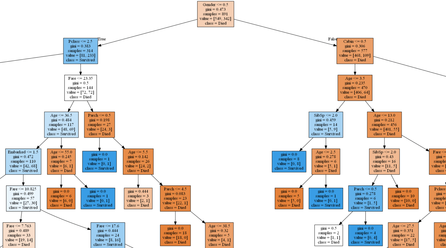
Excellent work! You have now implemented the heart of the decision tree learning algorithm. This function provides the mechanism for making a greedy, data-driven choice at each node to recursively partition the data.

Key Takeaways:

• Finding the best split is a search problem, which can be solved by iterating through all features and all possible thresholds.
• "Best" is defined as the split that maximizes information gain.
• The logic involves a nested loop structure: the outer loop for features and the inner loop for unique values (thresholds).
• The result of this function is the single question (e.g., "feature_X <= Y?") that most effectively purifies the dataset at a given node.

Preview of the Next Lesson:
We have all the essential components: a way to measure a split's quality (information_gain) and a way to find the best split (find_best_split). In the next lesson, we will tie everything together by building a recursive function to construct a full decision tree. This function will call find_best_split to create a node, and then it will call itself on the two resulting data subsets to create the child nodes, continuing until a stopping condition is met.