Hello! Welcome to the final lesson in our module on regularization.
In the previous lessons, you successfully implemented L1 (Lasso) and L2 (Ridge) regularization from scratch, modifying the cost functions and gradient calculations for your linear and logistic regression models. You now have the practical "how."
Today, we'll dive into the "why." This lesson focuses on comparing the effects of L1 and L2 regularization, specifically answering the crucial question: Why does L1 regularization lead to sparse models (i.e., set some coefficients to exactly zero), while L2 does not? Understanding this difference is key to choosing the right regularization strategy for a given problem. We'll explore this through visual, geometric, and gradient-based perspectives.
1. The Shape of the Penalty: A Visual Intuition
The fundamental difference between L1 and L2 regularization lies in the shape of their penalty functions. As a reminder:
- L2 (Ridge) Penalty: (a squared term)
- L1 (Lasso) Penalty: (an absolute value term)
When we add these penalties to our original loss function (like MSE, which is parabolic), the location of the new minimum changes in distinct ways. L2's squared penalty is also a parabola, so adding it to the MSE parabola results in another smooth parabola. Its minimum is shifted closer to zero, but it rarely lands exactly on it.
L1's absolute value penalty, however, is a 'V' shape. When you add a V-shape to a parabola, you can get a sharp "kink" at the bottom. For a strong enough regularization parameter lambda_, the lowest point of this new combined function can fall exactly at this kink, where the weight is zero.
The "StatQuest" video provides an excellent animated visualization of this exact process.
Ridge vs Lasso Regression, Visualized!!!
Watch this video from StatQuest with Josh Starmer to see how the L1 and L2 penalty functions, when added to the sum of squared residuals, affect the optimal slope.
Watch from 02:03 to 08:33. First, observe how the L2 penalty (Ridge) creates a new parabolic cost function whose minimum gets closer to zero but remains non-zero. Then, see how the L1 penalty (Lasso) creates a 'kink' at zero, allowing the minimum to land exactly at zero, effectively eliminating the feature. The final summary directly compares the two shapes.
2. The Geometric View: A Tale of a Diamond and a Circle
We can extend this intuition to a model with two weights, and . In this case, minimizing the regularized loss is equivalent to minimizing the original loss (e.g., MSE) subject to a constraint:
- L1 Constraint: . This defines a diamond shape in the weight space.
- L2 Constraint: . This defines a circle.
The unregularized loss function forms a set of concentric ellipses (contours) in the weight space. The optimal solution is the point where the loss contour first touches the constraint region.
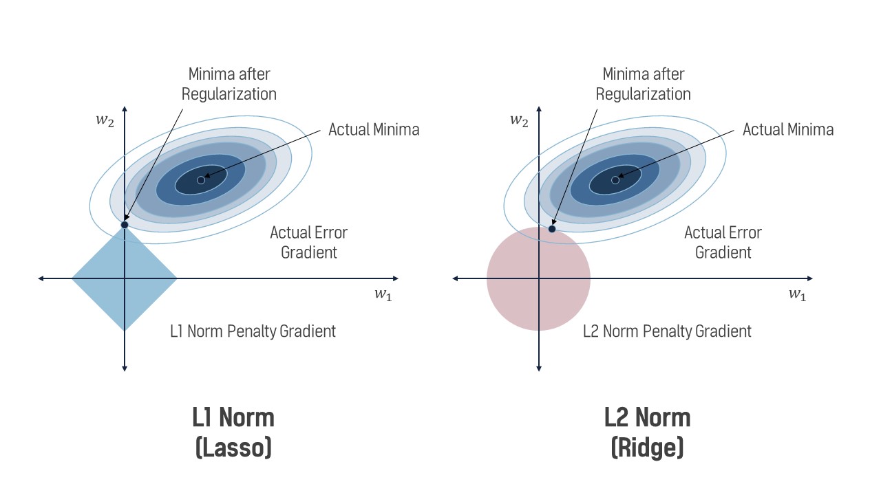
As you can see, the ellipses are more likely to touch the L1 diamond at one of its corners, which lie on the axes. A point on an axis means one of the weights is exactly zero. The L2 circle, being smooth, has no corners, so the contact point can be anywhere on its boundary, usually where both weights are non-zero.
This geometric view is a cornerstone of understanding regularization. The following resource provides a clear explanation of this visualization.
Elastic Net Regularization: Complete Guide
This article on Elastic Net regularization has an excellent section explaining the geometric view with a similar diagram.
Please read the section titled 'Geometric Interpretation of Regularization'. Focus on the visualization and the three bullet points below it that explain the L1 Constraint (Diamond), L2 Constraint (Circle), and the resulting effects on sparsity.
3. The Gradient's Perspective: A Constant Push vs. a Gentle Nudge
Since you have implemented the gradients yourself, let's connect this behavior directly to your code. The difference arises from the derivative of the penalty term.
-
Gradient of L2 penalty: . This term is proportional to the weight
w_jitself. As the weight gets smaller and approaches zero, the regularization gradient also shrinks to zero. It gives a gentle nudge, but the push weakens as you get closer to the target. -
Gradient of L1 penalty: . This term is constant! It's either or (or undefined at zero). This means that even when a weight is very small (e.g.,
0.0001), gradient descent still subtracts a fixed amount (learning_rate * \lambda / n) from it on every step. This constant, relentless push is what eventually forces the weight to cross the zero line and stay there.
The following article offers a great summary of this gradient-based reasoning.
A better visualization of L1 and L2 Regularization
Let's revisit an article that has another great explanation, this time focusing on the gradients.
Read the paragraph starting with 'Another way of thinking about this...'. It clearly contrasts the fixed gradient from L1 with the decreasing gradient from L2, providing the code-level intuition for why L1's 'push' towards zero doesn't weaken.
Test your understanding!
Imagine you have a model with a single weight, w = 0.01. Your learning rate is 0.01 and lambda_ / n_samples is 0.5.
- For L2 regularization, what is the value of the gradient update
learning_rate * l2_gradient_term? - For L1 regularization, what is the value of the gradient update
learning_rate * l1_gradient_term? - Based on these values, which method applies a stronger "push" towards zero when the weight is already very small?
Show answer
- L2 update: The gradient term is
(lambda_ / n) * w = 0.5 * 0.01 = 0.005. The update islearning_rate * 0.005 = 0.01 * 0.005 = 0.00005. - L1 update: The gradient term is
(lambda_ / n) * sign(w) = 0.5 * sign(0.01) = 0.5 * 1 = 0.5. The update islearning_rate * 0.5 = 0.01 * 0.5 = 0.005. - The L1 update (
0.005) is 100 times larger than the L2 update (0.00005). This demonstrates that L1 applies a much stronger, constant push towards zero, even for tiny weights, while the L2 push becomes negligible.
4. A Practical Experiment in Code
Let's prove this with the LinearRegression class you modified in the last lesson. We'll create a synthetic dataset where some features are useful and others are pure noise. Then we'll see which coefficients L1 and L2 regularization decide to keep.
Assuming your modified LinearRegression class from the previous lesson is saved in a file named linear_regression.py, you can run the following script:
import numpy as np
# Make sure your updated LinearRegression class is accessible
from linear_regression import LinearRegression

# 1. Generate synthetic data
# Let's create a dataset with 5 features.
# The target y will only depend on the first two features.
# The last three features are irrelevant noise.
np.random.seed(42)
X = np.random.rand(100, 5) * 10
# y = 3*X0 + 5*X1 + noise. True weights are [3, 5, 0, 0, 0]
y = 3 * X[:, 0] + 5 * X[:, 1] + np.random.randn(100) * 2

# 2. Train an L1 (Lasso) regularized model
# We use a relatively high lambda to encourage sparsity
lasso_model = LinearRegression(learning_rate=0.01, n_iters=1000, regularization='l1', lambda_=1.0)
lasso_model.fit(X, y)

# 3. Train an L2 (Ridge) regularized model
ridge_model = LinearRegression(learning_rate=0.01, n_iters=1000, regularization='l2', lambda_=1.0)
ridge_model.fit(X, y)

# 4. Compare the final weights
print("--- Comparing L1 and L2 Effects on Sparsity ---")
print(f"True weights should be close to: [3, 5, 0, 0, 0]\n")

print("L2 (Ridge) Coefficients:")
print(np.round(ridge_model.weights, 4))
print("--> Notice all coefficients are small but non-zero.\n")

print("L1 (Lasso) Coefficients:")
print(np.round(lasso_model.weights, 4))
print("--> Notice the last three coefficients are exactly zero!")
When you run this code, you should see that the L2 model assigns small, non-zero weights to all features. The L1 model, however, should drive the weights for the noisy features (the last three) all the way to zero, effectively performing automatic feature selection.
Conclusion
You have now explored the crucial differences between L1 and L2 regularization from multiple angles. This understanding elevates you from someone who can simply implement regularization to someone who can reason about when and why to use each type.
Key Takeaways:
| Aspect | L2 Regularization (Ridge) | L1 Regularization (Lasso) |
|---|---|---|
| Penalty Term | Adds sum of squared coefficients (). | Adds sum of absolute coefficients ($ |
| Geometric View | Circular constraint region. | Diamond-shaped constraint region. |
| Effect on Coeffs | Shrinks coefficients towards zero. | Can shrink coefficients exactly to zero. |
| Sparsity | Produces non-sparse solutions. | Produces sparse solutions. |
| Primary Use Case | When all features are potentially relevant; handles correlated features well. | For automatic feature selection; when many features may be irrelevant. |
Preview of the Next Module:
We have now completed our deep dive into linear models, optimization, and regularization. In the next module, we will explore a powerful and mathematically elegant approach to classification: Support Vector Machines (SVMs). We'll begin by building the intuition behind maximum margin classification and understanding the critical role of "support vectors" in defining a decision boundary.