Variational Method for Ground States

1. The Rayleigh-Ritz Variational Principle

At its heart, the variational method is built on a simple yet profound theorem. For any quantum system with a Hamiltonian $H$ and a true, but unknown, ground state energy $E_0$, the expectation value of the energy for any trial wavefunction $|\psi ⟩$ will always be greater than or equal to $E_0$.

As the reading shows, the proof is remarkably straightforward. Any trial state $|\psi ⟩={\sum }_n{a}_n|n⟩$ can be written as a superposition of the true energy eigenstates $|n⟩$. Its energy expectation value is:

Since $E_n\ge E_0$ for all $n$, we can replace each $E_n$ with $E_0$ to get the inequality:

Equality holds only if the trial state $|\psi ⟩$ is exactly the ground state $|0⟩$.

This theorem is powerful because it converts a difficult problem (solving the Schrödinger equation) into a more manageable one: an optimization problem. The strategy, known as the Rayleigh-Ritz method, is:

1. Guess a trial wavefunction $|\psi (\vec{\alpha })⟩$ that depends on one or more parameters $\vec{\alpha }$. This guess should be guided by physical intuition about the system's symmetries and expected behavior.
2. Calculate the energy expectation value $E(\vec{\alpha })=⟨\psi (\vec{\alpha })|H|\psi (\vec{\alpha })⟩/⟨\psi (\vec{\alpha })|\psi (\vec{\alpha })⟩$.
3. Minimize the energy with respect to the parameters by solving $\frac{\partial E}{\partial {\alpha }_i}=0$.
4. The resulting minimum energy, $E({\vec{\alpha }}_{\text{min}})$, is the best possible upper bound on $E_0$ for that family of trial functions.

A key reason for the method's effectiveness is that a "good" guess for the wavefunction yields a "very good" estimate for the energy. An error of order $ϵ$ in the wavefunction leads to an error of only order ${ϵ}^2$ in the energy. You can see the formal proof for this in the next section of the same notes ([PDF] 2. Approximation Methods - DAMTP, subsection "How Accurate is the Variational Method?").

2. A First Example: The Harmonic Oscillator

Let's see this strategy in action. We'll estimate the ground state energy for the one-dimensional quantum harmonic oscillator (QHO), whose Hamiltonian is:

Of course, we know the exact answer is $E_0=\frac{1}{2}\hslash \omega$, which makes this a perfect test case. For our trial function, we won't use the correct Gaussian form. Instead, let's use a function that has the right general shape—peaked at zero and decaying—but is functionally different, to see how well the method works with an imperfect guess.

3. A Realistic Problem: The Helium Atom

The true power of the variational method is demonstrated on problems that cannot be solved exactly. A classic example is the ground state of the Helium atom, which consists of a nucleus with charge $Z=2$ and two electrons. The Hamiltonian is:

The final term, representing the electron-electron repulsion, prevents an exact solution.

What is a good trial wavefunction? A simple first guess might be to ignore the repulsion term and just use two independent hydrogen ground state wavefunctions. This is precisely what we do in first-order perturbation theory. The variational method allows us to improve this guess. The physical insight is that one electron will screen the nuclear charge seen by the other electron. We can model this by using a trial wavefunction built from hydrogenic orbitals, but with an effective nuclear charge $\alpha$ that we treat as a variational parameter instead of fixing it at $Z=2$.

The calculation yields an optimal effective charge of $\alpha =Z-5/16=27/16\approx 1.69$. This result is beautifully intuitive: the presence of the other electron reduces the effective nuclear charge from 2 to about 1.69. Plugging this back into the energy formula gives an estimate of $E\approx -77.5\text{eV}$. This is a significant improvement over the first-order perturbation theory result ($-74.8\text{eV}$) and is remarkably close to the experimental value of $-79.0\text{eV}$.

4. Modern Application: The Variational Quantum Eigensolver

The variational principle is not just a historical tool from the annals of quantum mechanics; it is the engine behind some of the most promising algorithms for near-term quantum computers. One such algorithm is the Variational Quantum Eigensolver (VQE), which is used to find ground state energies of molecules and materials—a central problem in quantum chemistry and condensed matter physics.

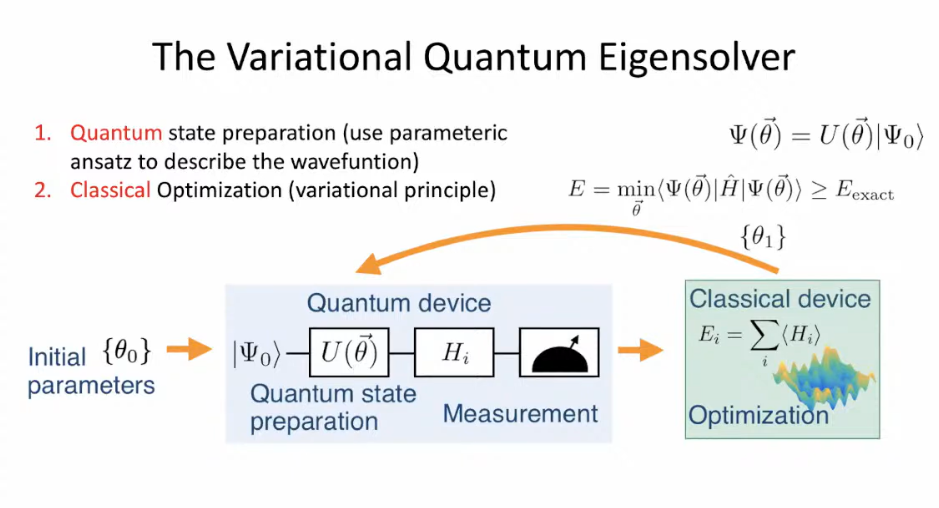
The VQE algorithm is a direct analogue of the Rayleigh-Ritz method:

1. Trial State: Instead of a mathematical function, the trial state $|\Psi (\vec{\theta })⟩$ is prepared on a quantum computer using a sequence of quantum gates with tunable parameters $\vec{\theta }$ (e.g., rotation angles). This is called a "parametric ansatz".
2. Energy Calculation: The quantum computer measures the expectation value of the Hamiltonian, $⟨H⟩$, for the prepared state. This is typically done by measuring the expectation values of individual terms in $H$ (like Pauli strings) and summing them classically.
3. Minimization: The measured energy is fed to a classical optimization algorithm (e.g., gradient descent) running on a classical computer. The optimizer's job is to suggest the next set of parameters $\vec{\theta }$ that will lower the energy.

This loop is repeated until the energy converges to a minimum. This hybrid quantum-classical approach leverages the quantum computer's ability to efficiently represent complex quantum states while using robust classical methods for the optimization task. It's a powerful modern testament to the enduring relevance of the variational principle you've just learned.

Conclusion

Today, we've added a powerful non-perturbative tool to your methodology toolkit. Unlike perturbation theory, the variational method provides a rigorous upper bound for the ground state energy and relies on physical intuition and optimization rather than a small expansion parameter.

Key Takeaways:

• The Variational Theorem: The expectation value of the energy for any trial state is always greater than or equal to the true ground state energy.
• The Rayleigh-Ritz Strategy: A problem is solved by guessing a physically motivated, parameterized trial wavefunction, calculating its energy expectation value, and minimizing this energy with respect to the parameters.
• Accuracy: The method is often highly accurate because an error of order $ϵ$ in the trial wavefunction results in a much smaller error of order ${ϵ}^2$ in the energy estimate.
• Physical Insight: The optimal values of the variational parameters can provide direct physical insight, such as the concept of charge screening in the Helium atom.
• Modern Relevance: The principle is the foundation for hybrid quantum-classical algorithms like VQE, which are at the forefront of quantum computation for chemistry and materials science.

The quality of a variational estimate depends entirely on how well the chosen family of trial functions can approximate the true ground state. This raises a crucial question: how do we assess the quality and reliability of our approximations? In our next lesson, we will delve into methods for assessing the domain of validity for any approximation, a critical skill for a practicing theorist.