Welcome back. The previous lesson showed why a party can lose seats because its supporters live close together, even when no one draws boundaries to disadvantage it. That leaves a practical question: if geography and ordinary districting rules already affect the result, how can you tell whether one particular map has an unusual partisan outcome?
This lesson introduces map ensembles: collections of alternative plans drawn for the same electorate under stated constraints. You will use one to judge how unusual a seat result is, then separate that judgment from any claim about the mapmakers’ intentions. Allow about 40 minutes for the short video, two readings, and the worked comparison.
Compare the map with alternatives, not an imagined blank slate
A map that gives one party far fewer seats than its statewide vote share might suggest could reflect residential geography, deliberate line-drawing, or both. An ensemble makes the comparison more specific: keep the voters and the election data fixed, generate many alternative district maps under a defined set of rules, and count the seats each map would produce.
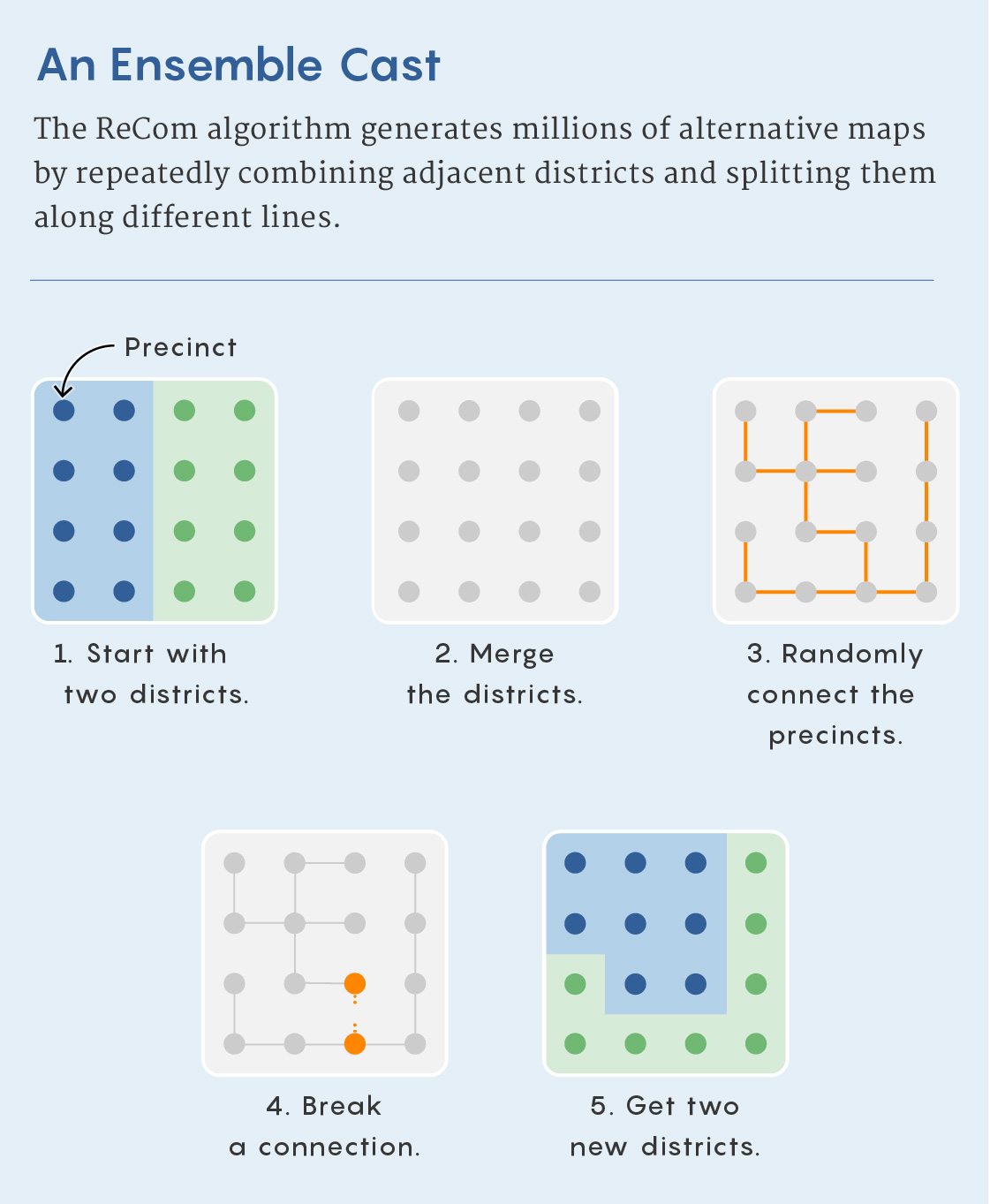
The following image illustrates one way to generate alternatives. In the ReCom approach, a pair of neighboring districts is combined, connections between their precincts are sampled, and the combined area is split again. In practice, proposed splits must be checked against requirements such as population balance. Repeating the operation produces many maps; it does not mean that every possible valid map is equally likely to appear.
Watch this brief explanation of what an ensemble comparison is intended to show. Listen especially carefully to how strongly the narrator interprets an outlier; we will qualify that claim below.
The algorithm that could help end partisan gerrymandering
Vox’s “The algorithm that could help end partisan gerrymandering” introduces map-drawing constraints and the idea of comparing a disputed plan with simulated alternatives.
Watch map constraints for the inputs used to generate alternatives, then the comparison for the outlier argument. The narrator calls the comparison “proof” of political bias; for this lesson, treat that as a claim to scrutinize, not a conclusion established by the simulation alone.
The central idea is sound but conditional: unusual relative to which alternatives? An ensemble is useful only insofar as its rules represent a relevant set of maps that could have been drawn.
Build a meaningful baseline
Population requirements, contiguity, treatment of county boundaries, geographic shape, and protections for minority voters can all change which maps enter an ensemble. These are not cosmetic choices. If a rule excludes maps that would otherwise elect more of one party’s candidates, the resulting seat distribution changes too.
Read how one project constructs its baseline and defines an outlier range.
Redistricting Report Card Methodology | Gerrymandering Project
Read the Princeton Gerrymandering Project’s methodology to see both how its alternative maps are constrained and how it compares their seat outcomes.
In the methodology discussion immediately before the “Partisan Fairness” heading, read the ensemble setup. Start at the paragraph about possible alternative plans and stop after the paragraph on calculating Democratic and competitive districts. Then, under “Partisan Fairness,” read the comparison rule in its first two paragraphs. Focus on the difference between the ensemble’s seat range and the separate vote-share-based fairness benchmark.
This project uses the middle 90% of simulated seat outcomes—between the 5th and 95th percentiles—as one comparison range. Its report card also considers an aspirational range based on statewide vote share. Those are different questions. A plan can be typical of the simulated maps yet yield seats that look disproportionate to the statewide vote, especially if residential geography affects many of the alternatives.
There is no single constraint set shared by every simulation. The Princeton methodology, for example, specifies a population tolerance and limits on splits for its ensemble; those settings should not be mistaken for universal requirements. Another research team describes how it translates criteria into hard constraints, which sampled plans must satisfy, and soft constraints, which favor some plans without excluding all others.
Simulated redistricting plans for the analysis and evaluation of ...
Read the “Methods” section of Imai and colleagues’ study to see why an ensemble’s design matters to the conclusion drawn from it.
In “Methods” (pp. 2–3), begin with the paragraph about the state receiving 14 congressional districts and read the criteria and example, stopping after the explanation of the soft minority-representation target. Next, on p. 3, read hard and soft constraints; stop before the paragraph beginning “Additionally, we add a hard constraint.” Notice that the researchers say which criterion their simulations omit as well as which ones they model.
The researchers’ explicit omission of a criterion—avoiding unnecessary pairing of incumbents—illustrates a general limit. A simulated map may satisfy every rule in the model without satisfying every consideration that mattered to the people who drew the actual plan. Conversely, a claimed constraint should not be accepted merely because it helps explain away an unusual result. Evaluating the comparison means inspecting both the stated rules and how they were implemented.
Work through an ensemble result
Suppose a hypothetical state has five districts. For this example, assume that all 100 alternative maps use the same precinct-level election results, give each party the same voters and preferences, and satisfy the stated rules: contiguous districts, the required population balance, a county-split limit, a specified compactness standard, and applicable minority-representation constraints. Across those fixed election results, Party D receives 52% of the statewide vote.
Here is the supplied ensemble’s distribution of Party D seats:
| Party D seats | Number of alternative maps |
|---|---|
| 1 | 2 |
| 2 | 18 |
| 3 | 45 |
| 4 | 33 |
| 5 | 2 |
| Total | 100 |
Suppose the map being evaluated also elects one Party D candidate under those election results. Only 2 of the 100 alternatives do as poorly for D: its observed lower-tail frequency is . In this example, the 5th-percentile outcome is two seats, while the 95th-percentile outcome is four seats. The evaluated map’s one-seat result falls below that middle-90% range.
That supports a precise statement: under these election data, constraints, and sampling method, the map produces a Party D seat outcome that is unusual relative to the supplied alternatives. It does not establish that Party D “should” receive exactly 52% of five seats, nor that three seats is the uniquely fair result. The ensemble answers a question about available map choices, not a universal question about proportional representation.
It also does not turn into “a 98% probability that the mapmakers intended to disadvantage Party D.” The fraction describes simulated map outcomes. It is not a measurement of anyone’s motives. An unusually low result makes the boundary choices worth closer examination; evidence about how and why those choices were made is a separate matter.
Read an ensemble plot without losing the comparison
Real displays may show several election scenarios rather than a single table. In the chart below, the horizontal axis gives the number of Democrats elected and the vertical axis gives statewide Democratic vote percentage. Orange distributions show the range of alternative-map outcomes at particular vote levels; colored points mark outcomes for specific plans.

Near 50.88% on the vertical axis, for example, the colored points sit at different seat counts. Their horizontal separation shows that maps can yield different representation under a similar statewide vote. To assess whether one point is unusual, though, you need its position within the relevant orange distribution—not just its distance from another colored point.
The chart alone does not tell you every constraint used to generate those alternatives, how the election results were applied to each map, or whether a small-looking tail contains many sampled maps. A visual impression of an outlier is a starting point for an assessment, not a substitute for the ensemble’s specifications and counts.
State what the result can—and cannot—show
An ensemble comparison is especially informative when it holds the electorate and election assumptions constant while varying the boundaries. It helps separate an outcome common to many permissible maps—which might reflect residential geography and constraints—from an outcome reached by relatively few of them. But its force depends on the baseline:
- Constraints: Were the relevant population, geographic, and voting-rights criteria modeled appropriately?
- Sampling: Did the method explore a sufficiently broad and stable range of permissible maps? A million generated maps are not automatically a million independent or equally likely possibilities.
- Election assumptions: Were the same election data applied consistently? Historical precinct votes can illustrate how maps perform under that election; they do not guarantee future results.
- Interpretation: Is the claim about an unusual seat outcome, or about intent? The first can be measured against an ensemble. The second needs additional evidence.
These qualifications do not make the comparison useless. They make its conclusion more defensible. If a result remains far outside the alternatives under reasonable, clearly stated choices of constraints and election data, that is stronger evidence of an exceptional map outcome than a statewide vote-to-seat comparison alone. It is still not, by itself, proof of partisan manipulation.
Key takeaways
To evaluate a map against an ensemble, first identify the rules and election data used to generate the alternatives. Then compare its seat count with the distribution—ideally reporting a range or tail frequency rather than simply calling it an outlier. Unusual relative to comparable maps is a meaningful finding; drawn with partisan intent is a further claim that the seat distribution alone cannot settle.
The next lesson turns to where a partisan-gerrymandering challenge can be brought after Rucho v. Common Cause, including why federal and state legal routes need to be distinguished.