Comparing Oracle and Sample-Covariance Minimum-Variance Portfolios in Python

What exactly are we comparing?

Let the data-generating process be

where $\Sigma$ is a known positive-definite population covariance matrix. We set the mean to zero because the GMV portfolio does not use expected returns.

The oracle GMV weights are

From one simulated training sample, we estimate

and construct the sample-covariance GMV portfolio,

Both portfolios are fully invested:

They differ only in whether the covariance input is known or estimated.

The key evaluation rule is this:

Evaluate both sets of weights using the true covariance matrix $\Sigma$, not the sample covariance used to construct them.

Thus the oracle’s population variance is

whereas the sample portfolio’s true, or ex-ante, variance is

Because ${\mathbf{w}}_{\star }$ is the population GMV solution,

More precisely, the excess variance is

This identity is especially useful. It says that the decision loss from using the sample covariance is exactly the covariance-weighted squared distance between the estimated and oracle weight vectors.

A second quantity is deliberately misleading if treated as a forecast:

This is the portfolio’s in-sample variance. It is low partly because $\hat{\mathbf{w}}$ was selected specifically to minimize that same sample quantity. Across simulations, it tends to understate the portfolio’s true risk: an instance of optimizer’s in-sample optimism.

A simulation protocol used in covariance-estimation research

The useful feature of a Monte Carlo setting is not merely that it is artificial; it gives us an otherwise unavailable benchmark, $\Sigma$. Coqueret and Milhau use this setup to measure the increase in ex-ante volatility incurred when a minimum-variance portfolio uses an estimated covariance matrix rather than the known population matrix.

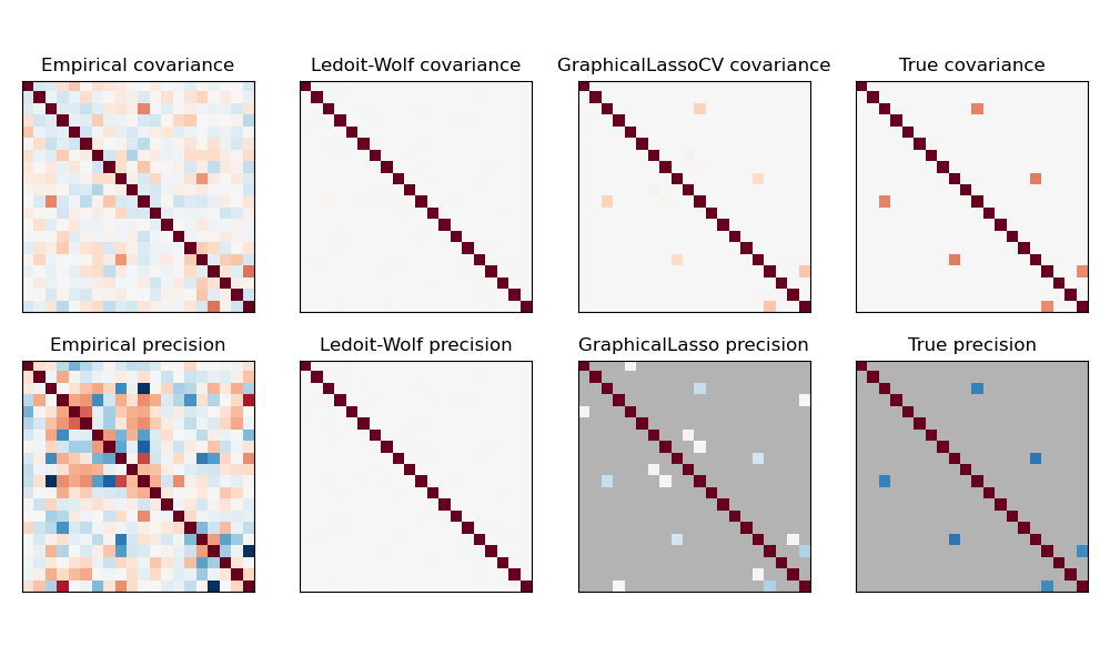
The image below gives a visual version of the central issue. The empirical covariance is visibly more irregular than the true covariance, and the corresponding empirical precision matrix—its inverse—is much noisier still. In the present lesson we use only the empirical and true matrices; the middle columns preview regularized estimators that will be studied later.

Build a population covariance and the oracle portfolio

A diagonal $\Sigma$ would be a valid first experiment, but a one-factor covariance structure is more informative. It creates correlated assets with heterogeneous market exposures and idiosyncratic volatilities:

where $D$ is diagonal and positive. This is a simple population model, not a claim that real returns are exactly one-factor Gaussian.

The code below creates the population covariance, draws Gaussian returns, and implements GMV weights. Notice that the code uses np.linalg.solve rather than forming a matrix inverse explicitly. Algebraically,

and the solution of

are the same vector, but solving the linear system is numerically preferable.

import numpy as np
import pandas as pd
import matplotlib.pyplot as plt


def make_factor_covariance(n_assets, rng):
    """
    Construct a positive-definite one-factor population covariance matrix.
    Units are daily return units.
    """
    beta = rng.uniform(0.4, 1.4, size=n_assets)
    idio_vol = rng.uniform(0.006, 0.020, size=n_assets)
    market_vol = 0.010

    sigma = (
        market_vol**2 * np.outer(beta, beta)
        + np.diag(idio_vol**2)
    )
    return sigma


def draw_gaussian_returns(T, sigma, rng):
    """Draw T i.i.d. zero-mean Gaussian return vectors with covariance sigma."""
    n_assets = sigma.shape[0]
    chol = np.linalg.cholesky(sigma)
    z = rng.standard_normal((T, n_assets))
    return z @ chol.T


def gmv_weights(covariance):
    """
    Unconstrained fully invested GMV weights.

    This function assumes covariance is positive definite.
    """
    n_assets = covariance.shape[0]
    ones = np.ones(n_assets)

    numerator = np.linalg.solve(covariance, ones)
    weights = numerator / (ones @ numerator)

    return weights


def portfolio_volatility(weights, covariance):
    """Population or estimated volatility, depending on covariance supplied."""
    variance = weights @ covariance @ weights
    return np.sqrt(variance)

Now fix a single population covariance matrix. It must remain fixed as we vary $T$; otherwise a change in results could reflect a change in the underlying investment universe rather than sampling uncertainty.

rng_population = np.random.default_rng(2025)

N = 40
Sigma = make_factor_covariance(N, rng_population)

w_oracle = gmv_weights(Sigma)
oracle_vol = portfolio_volatility(w_oracle, Sigma)

print(f"Oracle daily volatility: {oracle_vol:.4%}")
print(f"Oracle weight sum:      {w_oracle.sum():.12f}")
print(f"Oracle gross exposure:  {np.abs(w_oracle).sum():.3f}")

The gross exposure,

equals one for a long-only fully invested portfolio. Values above one reveal offsetting long and short positions. Such positions are allowed in the unconstrained GMV solution used here, and they are often where estimation error becomes economically consequential.

One training sample: apparent risk versus true risk

Before averaging over many samples, inspect one estimation window. We choose $T=67$, giving

The sample covariance is nonsingular because $N<T$, but this is still a relatively demanding estimation problem.

rng_one_sample = np.random.default_rng(73)

T = 67
returns = draw_gaussian_returns(T, Sigma, rng_one_sample)

# np.cov centers each return series and uses the T - 1 denominator by default.
S = np.cov(returns, rowvar=False, ddof=1)

w_sample = gmv_weights(S)

sample_in_vol = portfolio_volatility(w_sample, S)
sample_true_vol = portfolio_volatility(w_sample, Sigma)

riv_one_sample = sample_true_vol / oracle_vol - 1.0
weight_error = np.linalg.norm(w_sample - w_oracle)

print(f"q = N / T:                    {N / T:.3f}")
print(f"Oracle true volatility:        {oracle_vol:.4%}")
print(f"Sample portfolio in-sample:    {sample_in_vol:.4%}")
print(f"Sample portfolio true risk:    {sample_true_vol:.4%}")
print(f"Relative increase in vol:      {riv_one_sample:.2%}")
print(f"Weight L2 error:               {weight_error:.3f}")
print(f"Sample gross exposure:         {np.abs(w_sample).sum():.3f}")

Interpret the three volatility lines carefully:

• Oracle true volatility is the smallest attainable population volatility under the full-investment constraint.
• Sample portfolio in-sample volatility is what the optimizer reports from the training covariance matrix.
• Sample portfolio true risk is the relevant quantity in this controlled experiment: the risk that the same sample-derived weights have under the true $\Sigma$.

The in-sample figure may look impressive, but it is not an independent validation. The optimizer searched over many weight vectors and chose one that exploits favorable features—including accidental ones—of that particular sample covariance matrix.

Monte Carlo comparison across dimensional ratios

A single training sample can be unusually benign or unusually bad. The appropriate comparison repeats the experiment many times while holding $\Sigma$, $N$, and the portfolio rule fixed.

We vary the target dimensional ratio by changing only the number of observations $T$. All values remain below one, so the standard sample covariance is invertible with probability one under this continuous Gaussian model. The $q\approx 0.8$ case is nonetheless close enough to the singular boundary to show substantial inverse-covariance sensitivity.

def run_monte_carlo(sigma, q_targets, n_replications, seed=1234):
    """
    Compare sample-covariance GMV portfolios with the oracle GMV portfolio
    over repeated Gaussian training samples.
    """
    rng = np.random.default_rng(seed)
    n_assets = sigma.shape[0]

    w_oracle = gmv_weights(sigma)
    oracle_vol = portfolio_volatility(w_oracle, sigma)

    records = []

    for q_target in q_targets:
        # T > N is required because sample covariance uses mean centering.
        T = int(np.ceil(n_assets / q_target))
        if T <= n_assets:
            raise ValueError("Choose q_target below 1 for this experiment.")

        for replication in range(n_replications):
            returns = draw_gaussian_returns(T, sigma, rng)
            sample_cov = np.cov(returns, rowvar=False, ddof=1)

            w_sample = gmv_weights(sample_cov)

            in_sample_vol = portfolio_volatility(w_sample, sample_cov)
            true_vol = portfolio_volatility(w_sample, sigma)

            records.append(
                {
                    "q": n_assets / T,
                    "T": T,
                    "replication": replication,
                    "in_sample_vol": in_sample_vol,
                    "true_vol": true_vol,
                    "riv": true_vol / oracle_vol - 1.0,
                    "weight_l2_error": np.linalg.norm(w_sample - w_oracle),
                    "gross_exposure": np.abs(w_sample).sum(),
                }
            )

    return pd.DataFrame(records), w_oracle, oracle_vol


q_targets = [0.10, 0.30, 0.60, 0.80]

results, w_oracle, oracle_vol = run_monte_carlo(
    Sigma,
    q_targets=q_targets,
    n_replications=400,
    seed=91,
)

summary = (
    results.groupby(["q", "T"], as_index=False)
    .agg(
        mean_in_sample_vol=("in_sample_vol", "mean"),
        mean_true_vol=("true_vol", "mean"),
        mean_riv=("riv", "mean"),
        sd_riv=("riv", "std"),
        mean_weight_l2_error=("weight_l2_error", "mean"),
        mean_gross_exposure=("gross_exposure", "mean"),
    )
    .sort_values("q")
)

summary["oracle_vol"] = oracle_vol
summary["mean_riv_pct"] = 100 * summary["mean_riv"]
summary["sd_riv_pct"] = 100 * summary["sd_riv"]

display_columns = [
    "q",
    "T",
    "oracle_vol",
    "mean_in_sample_vol",
    "mean_true_vol",
    "mean_riv_pct",
    "sd_riv_pct",
    "mean_gross_exposure",
]

print(summary[display_columns].round(4).to_string(index=False))

Plot the most decision-relevant results.

fig, axes = plt.subplots(1, 3, figsize=(15, 4))

# True and in-sample volatility
axes[0].plot(
    summary["q"],
    summary["mean_true_vol"],
    marker="o",
    label="Sample portfolio: true volatility",
)
axes[0].plot(
    summary["q"],
    summary["mean_in_sample_vol"],
    marker="o",
    label="Sample portfolio: in-sample volatility",
)
axes[0].axhline(
    oracle_vol,
    color="black",
    linestyle="--",
    label="Oracle true volatility",
)
axes[0].set_xlabel("Dimensional ratio q = N / T")
axes[0].set_ylabel("Daily volatility")
axes[0].set_title("Risk forecast versus true risk")
axes[0].legend()

# Relative increase in true volatility
axes[1].plot(
    summary["q"],
    summary["mean_riv_pct"],
    marker="o",
    color="tab:red",
)
axes[1].set_xlabel("Dimensional ratio q = N / T")
axes[1].set_ylabel("Mean relative increase in volatility (%)")
axes[1].set_title("Cost of sample covariance")

# Gross exposure
axes[2].plot(
    summary["q"],
    summary["mean_gross_exposure"],
    marker="o",
    color="tab:purple",
)
axes[2].axhline(
    np.abs(w_oracle).sum(),
    color="black",
    linestyle="--",
    label="Oracle gross exposure",
)
axes[2].set_xlabel("Dimensional ratio q = N / T")
axes[2].set_ylabel("Mean gross exposure")
axes[2].set_title("Weight leverage from estimation")
axes[2].legend()

plt.tight_layout()
plt.show()

How to interpret the results

Your numerical values depend on the fixed population covariance and random seed, but the expected pattern is robust.

1. The sample portfolio’s true volatility rises with $q$

As $q$ increases, fewer observations are available per asset. The entries, eigenvalues, and eigenvectors of $\hat{\Sigma }$ become less accurately estimated. The resulting inverse covariance magnifies error, so the sample GMV portfolio generally has a larger population volatility than the oracle GMV portfolio.

The most direct performance measure is the relative increase in volatility:

This evaluates the portfolio decision, not merely the covariance estimate. A covariance estimator can have a seemingly modest matrix error while still inducing damaging GMV weights.

2. In-sample risk is too optimistic

The difference between mean_in_sample_vol and mean_true_vol is the practical warning sign. The sample GMV portfolio uses $\hat{\Sigma }$ both to choose the weights and to report their risk. This reuses the same noise twice.

In a real setting, $\Sigma$ is unknown, so you cannot calculate true risk exactly. You must instead use a properly separated future test period or a walk-forward backtest. Here, because the simulation supplies $\Sigma$, the true-risk evaluation is exact conditional on the weights.

3. Weight instability often accompanies poor risk outcomes

As $q$ approaches one, gross exposure typically rises. The optimizer finds apparently low-variance directions in the sample, frequently expressed through large offsetting long and short positions. Those directions need not be low risk under the true covariance.

This is the portfolio-level manifestation of the spectral point from earlier lessons:

A small underestimated sample eigenvalue ${\hat{\lambda }}_i$ receives a large inverse weight $1/{\hat{\lambda }}_i$. The optimizer can then overcommit to an unstable sample eigenvector direction.

4. Do not extend this raw experiment to $q\ge 1$

For the conventional mean-centered sample covariance,

implies singularity. The code therefore intentionally refuses $q\ge 1$. Replacing solve with a pseudoinverse would produce some weights, but it would silently change the portfolio rule by regularizing or discarding null-space directions. That is a distinct modelling decision, not a valid raw-sample benchmark.

A useful validation: fresh simulated returns

Although true covariance evaluation is exact in a simulation, it is useful to verify the connection with realized out-of-sample risk. For the w_sample from the earlier single-window example, draw a large independent test sample.

rng_test = np.random.default_rng(999)

T_test = 100_000
test_returns = draw_gaussian_returns(T_test, Sigma, rng_test)

realized_test_vol = test_returns @ w_sample
realized_test_vol = realized_test_vol.std(ddof=1)

print(f"Analytic true volatility: {sample_true_vol:.4%}")
print(f"Large-test-sample vol:    {realized_test_vol:.4%}")

With a sufficiently large test sample, the realized volatility should be close to

For a realistic short test period, the realized result would itself be noisy. That distinction will matter when the course moves from controlled simulations to walk-forward evaluation on financial data.

Takeaways

• The oracle GMV portfolio uses the true covariance $\Sigma$; the sample GMV portfolio replaces it with $\hat{\Sigma }$.
• In a Gaussian simulation, $\Sigma$ is known by construction, so it can evaluate each portfolio’s true risk exactly.
• The relevant cost of estimation is the sample portfolio’s excess population risk:

• The sample portfolio’s in-sample volatility is generally overoptimistic because the same covariance sample is used for optimization and evaluation.
• As $q=N/T$ increases toward one, raw sample-covariance GMV portfolios typically show higher true risk, larger weight error, and greater gross exposure.
• Use np.linalg.solve, not an explicit inverse, but recognize that numerical technique does not cure statistical estimation error.

The next module shifts from the portfolio consequence back to the random matrix itself: you will express a Gaussian sample covariance matrix as a scaled Wishart matrix and begin studying its eigenvalue distribution.