Deriving Global Minimum-Variance Portfolio Weights

The optimization problem

Suppose there are $N$ risky assets, with portfolio-weight vector

and covariance matrix $\Sigma$. Let $1$ denote the $N$-vector of ones.

A portfolio’s variance is

The full-investment constraint is

This means the weights sum to one. It allows short positions: for example, weights of $1.2$ and $-0.2$ still satisfy full investment because their net investment is one. We are not yet imposing long-only, leverage, turnover, or concentration constraints.

The GMVP solves

Two features distinguish this from the usual mean-variance problem:

1. Expected returns do not enter. The GMVP uses only covariance information.
2. “Global” means global over the feasible fully invested portfolios, not merely the least-volatile individual asset.

For the derivation, assume $\Sigma$ is symmetric positive definite. Thus it is invertible and the variance objective is strictly convex, giving a unique minimizer.

Deriving the GMVP weights

It is convenient to place a factor of $1/2$ in the objective. It does not change the minimizer, but it removes an unnecessary factor of two when differentiating:

Define the Lagrangian

The multiplier $\lambda$ enforces the full-investment constraint. Because $\Sigma$ is symmetric,

The first-order condition with respect to $\mathbf{w}$ is therefore

Rearrange:

Since $\Sigma$ is invertible,

This has an important interpretation: before normalization, the minimum-variance direction is ${\Sigma }^{-1}1$. The remaining task is to choose $\lambda$ so that this direction becomes a fully invested portfolio.

Apply the constraint:

Hence,

Substitution gives the central result:

The numerator determines the relative allocations implied by the covariance structure. The scalar denominator normalizes them so that their sum is exactly one.

Why this is truly the minimum

The first-order conditions identify a candidate. Positive definiteness of $\Sigma$ shows it is the unique global optimum.

Let ${\mathbf{w}}_{\star }$ denote the GMVP weights, and consider any other fully invested portfolio:

where the perturbation $\mathbf{u}$ preserves the budget constraint:

Its variance is

From the first-order condition,

Thus the cross term is

So

Since $\Sigma$ is positive definite, the final term is positive for every nonzero $\mathbf{u}$. Any feasible departure from ${\mathbf{w}}_{\star }$ therefore raises variance.

The corresponding minimum achievable variance also has a useful closed form:

This follows by substituting the optimal weights into ${\mathbf{w}}^{\mathsf{T}}\Sigma \mathbf{w}$.

Geometric meaning: the leftmost feasible portfolio

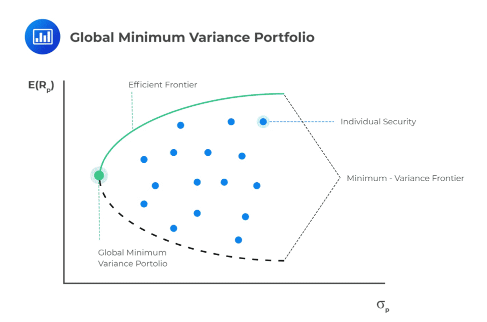
The diagram places expected return on the vertical axis and volatility on the horizontal axis. Every dot or interior point represents a feasible portfolio formed from the available assets.

The GMVP is the point with the smallest horizontal coordinate: no other fully invested combination can have a lower standard deviation. It need not have an especially high expected return, because the optimization has deliberately ignored expected returns.

Only the upper segment of the minimum-variance frontier is normally called mean-variance efficient: above the GMVP, higher expected return is paired with higher minimum achievable risk. The lower segment is inefficient because a portfolio on the upper branch can be found with the same risk and a higher expected return.

A two-asset example

For two assets, write

The GMVP weight in asset 1 is

and the weight in asset 2 is

Consider annualized quantities:

The covariance is

so

The GMVP weights are

The lower-volatility asset receives the larger allocation, but not $100\%$. Imperfect correlation creates diversification value, making a mix less risky than the first asset on its own.

The portfolio’s variance is

and its annualized volatility is approximately

That is below asset 1’s standalone volatility of $15\%$.

Reliable Python implementation

The formula is written with ${\Sigma }^{-1}$, but numerical code should normally solve a linear system rather than explicitly form an inverse. It is both more stable and more efficient.

import numpy as np

def gmv_weights(cov):
    """
    Global minimum-variance weights with a full-investment constraint.
    Short positions are permitted.
    """
    cov = np.asarray(cov, dtype=float)
    n_assets = cov.shape[0]
    ones = np.ones(n_assets)

    # x = Sigma^{-1} 1, computed without explicitly inverting Sigma
    x = np.linalg.solve(cov, ones)

    return x / (ones @ x)


cov = np.array([
    [0.0225, 0.0075],
    [0.0075, 0.0625]
])

w_gmv = gmv_weights(cov)
var_gmv = w_gmv @ cov @ w_gmv
vol_gmv = np.sqrt(var_gmv)

print("GMVP weights:", w_gmv)
print("Sum of weights:", w_gmv.sum())
print("GMVP variance:", var_gmv)
print("GMVP volatility:", vol_gmv)

The key outputs should be approximately:

GMVP weights: [0.78571429 0.21428571]
Sum of weights: 1.0
GMVP variance: 0.019285714285714285
GMVP volatility: 0.13887301496588272

A minimal implementation checklist is:

• Ensure cov is square and symmetric up to numerical tolerance.
• Check that it is sufficiently well conditioned before trusting its inverse-based weights.
• Verify that w_gmv.sum() is numerically close to one.
• Compute the implied variance as w_gmv @ cov @ w_gmv.

The connection to random matrix theory

The GMVP formula makes the eventual RMT problem visible immediately. If the covariance matrix has eigendecomposition

then

Each eigenvector direction is weighted by $1/{\lambda }_i$. Consequently, small estimated eigenvalues receive disproportionately large influence in GMVP weights. If those small eigenvalues arise partly from sampling noise—as they often do when the number of assets is not small relative to the return-history length—the resulting allocations can be unstable and extreme.

That is the motivation for the rest of this course: covariance cleaning is not merely about making a spectrum look smoother. It changes the inverse covariance matrix that directly determines risk-minimizing portfolio weights.

Key takeaways

• The GMVP minimizes ${\mathbf{w}}^{\mathsf{T}}\Sigma \mathbf{w}$ subject only to $1^{\mathsf{T}}\mathbf{w}=1$.
• Under an invertible positive-definite covariance matrix and unconstrained shorting,

• Its minimum variance is

• The inverse covariance is the critical object: small eigenvalues can exert a large effect on optimized weights.

Next, we will add expected returns and derive the unconstrained mean-variance portfolio for a chosen risk-aversion parameter.