Why Inversion Amplifies Error Along Low-Variance Eigenvectors

Inversion in the eigenvector basis

Let the estimated covariance matrix have eigendecomposition

where:

• ${\hat{\lambda }}_i>0$ is sample eigenvalue $i$;
• ${\hat{\mathbf{q}}}_i$ is its associated unit sample eigenvector;
• the eigenvectors form an orthonormal basis.

Inverting the matrix leaves the eigenvectors unchanged but reciprocates every eigenvalue:

This one operation is the core issue:

For any vector $\mathbf{b}$, inversion acts as

So the projection of $\mathbf{b}$ on eigenvector $i$ is scaled by $1/{\hat{\lambda }}_i$.

For the two optimizers already encountered:

and the unnormalized GMV direction is

The optimizer therefore does not merely use the covariance estimate. It gives the largest leverage to its least-variance directions.

A qualification matters: a small eigenvalue only affects a particular solution if the relevant vector has a nonzero projection on its eigenvector. For mean–variance optimization, that vector is $\hat{\mathbf{\mu }}$; for GMV, it is $1$. In realistic, asymmetric covariance matrices, those projections are generally nonzero. Moreover, errors in the estimated eigenvectors themselves can create or alter those projections.

The geometric meaning: undoing a nearly collapsed direction

A covariance matrix describes the shape of return dispersion. Its eigenvectors are the principal directions of that shape; its eigenvalues are the variances along them.

• A large eigenvalue corresponds to a broad direction of return variation.
• A small eigenvalue corresponds to a narrow direction: a particular long–short combination of assets that appears to have little variance.

Inversion reverses these scalings. Along a direction with variance ${\hat{\lambda }}_i$, the inverse has scaling $1/{\hat{\lambda }}_i$. Thus, a direction that the sample covariance says is almost flat gets magnified enormously.

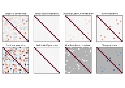
A useful way to interpret a low-variance eigenvector is as a candidate relative-value or hedged spread. If two assets appear almost perfectly correlated, an offsetting long–short combination may appear to have extremely low historical risk. But “appears” is doing substantial work: the low sample variance can arise from limited observations and chance alignment, rather than from a persistently low-risk economic relationship.

The inversion treats that apparent hedge as unusually attractive. The optimizer may then establish a large long position in one asset and a large short position in another, precisely because their historical difference looked unusually quiet.

Why a small eigenvalue makes estimation error dangerous

Suppose the true variance in an eigenvector direction is $\lambda$, but we estimate

The inverse-eigenvalue error is exactly

When $\epsilon$ is small relative to $\lambda$, this is approximately

The factor $1/{\lambda }^2$ is the amplification mechanism. For the same absolute eigenvalue estimation error $\epsilon$, the error in the inverse is much greater when $\lambda$ is small.

For example, suppose two eigenvalues each have an absolute estimation error of $0.001$:

The smaller eigenvalue produces an inverse error one hundred times as large.

This becomes catastrophic if the estimated eigenvalue is close to zero. If the true value is $\lambda =0.002$ and the sample estimate is $\hat{\lambda }=0.001$, then

A downward error of only $0.001$ doubles the inverse scaling in that direction.

Matrix-level perturbation view

The same result holds without assuming that the true and estimated covariance matrices share eigenvectors. Let

where $\Delta$ is the covariance estimation error. The inverse perturbation identity is

Taking the spectral norm gives

For a positive-definite matrix,

Thus, whenever the smallest eigenvalue is small, both inverse norms can be large. Modest covariance-estimation error can therefore produce a large error in the precision matrix ${\Sigma }^{-1}$, and hence in optimized weights.

The related diagnostic is the condition number:

A large condition number means that the covariance matrix has directions with very different scales and is numerically and statistically sensitive to inversion. It does not prove that a portfolio is bad, but it is a warning that unconstrained inverse-covariance optimization deserves scrutiny.

A two-asset spread example

Consider two equally volatile assets with annual variance $0.04$, or annual volatility $20\%$, and correlation $\rho$:

Its orthonormal eigenvectors are

The first is the common movement direction; the second is the long–short spread direction. The eigenvalues are

Set $\rho =0.975$. Then

The spread direction has eighty times less estimated variance than the common direction. Its inverse scaling is correspondingly eighty times greater:

Now suppose expected excess returns are

There is only a small expected-return difference between the assets. Yet that difference has a projection onto the spread direction:

The mean–variance coefficient in the spread direction, before dividing by $\gamma$, is

By comparison, the coefficient in the common direction is only about $0.98$. The optimizer turns a mild $1\%$ expected-return difference into a dominant leveraged long–short bet, because the sample says that spread is almost riskless.

If correlation is re-estimated at $0.980$, a change of just $0.005$, then

The estimated variance of the spread falls by $20\%$, and its inverse scaling rises from $1000$ to $1250$. The optimal long–short tilt changes sharply even though the individual expected returns did not change.

The issue is not that a low-risk spread can never be real. The issue is that an optimizer acts with excessive confidence in a feature whose estimated magnitude and direction may be highly uncertain.

Eigenvector error is amplified too

Eigenvalue noise is only half of the problem. The estimated eigenvectors are also random:

in general.

Recall the sample mean–variance decomposition:

An error in ${\hat{\mathbf{q}}}_i$ affects both:

1. the projection ${\hat{\mathbf{q}}}_i^{\mathsf{T}}\hat{\mathbf{\mu }}$, determining how much expected return is attributed to that direction; and
2. the portfolio direction ${\hat{\mathbf{q}}}_i$, determining how that exposure is distributed over individual assets.

Division by a small ${\hat{\lambda }}_i$ magnifies both effects.

This is especially relevant when several small sample eigenvalues are close together. Their associated eigenspace may be estimable as a group, but the individual sample eigenvectors within it can rotate substantially from one estimation window to another. If an optimizer gives those vectors enormous coefficients, the asset-level weights can vary dramatically after a small change in the return sample.

Inspecting the mechanism in Python

The following code reproduces the two-asset example. It reports eigenvalues, the coefficient assigned to each principal direction, the resulting weights, and gross exposure.

import numpy as np

def cov_from_correlation(rho, variance=0.04):
    return variance * np.array([
        [1.0, rho],
        [rho, 1.0]
    ])

def spectral_mean_variance(mu, cov, gamma=1.0):
    """
    Return the mean-variance weights and their spectral decomposition.
    gamma only rescales all coefficients and weights.
    """
    eigvals, eigvecs = np.linalg.eigh(cov)  # ascending eigenvalues
    projections = eigvecs.T @ mu
    coefficients = projections / (gamma * eigvals)
    weights = eigvecs @ coefficients

    return eigvals, eigvecs, projections, coefficients, weights


mu = np.array([0.06, 0.05])

for rho in [0.975, 0.980]:
    cov = cov_from_correlation(rho)

    eigvals, eigvecs, projections, coeffs, w = spectral_mean_variance(
        mu=mu,
        cov=cov,
        gamma=1.0
    )

    print(f"\nCorrelation: {rho:.3f}")
    print("Eigenvalues:", eigvals)
    print("Condition number:", eigvals[-1] / eigvals[0])
    print("Expected-return projections:", projections)
    print("Spectral coefficients:", coeffs)
    print("Weights:", w)
    print("Gross exposure:", np.abs(w).sum())

You should observe the following pattern:

• Increasing correlation from $0.975$ to $0.980$ makes the smallest eigenvalue fall from $0.001$ to $0.0008$.
• The condition number increases.
• The coefficient on the low-variance spread direction becomes larger in magnitude.
• The portfolio becomes more leveraged long–short, even though expected returns are unchanged.

In applied work, monitor at least:

eigvals = np.linalg.eigvalsh(sample_cov)
condition_number = eigvals[-1] / eigvals[0]

print("Smallest eigenvalue:", eigvals[0])
print("Largest eigenvalue:", eigvals[-1])
print("Condition number:", condition_number)

This is a diagnostic, not a complete solution. A low eigenvalue may represent genuine structure, while a large condition number may partly reflect differences in asset volatilities. For correlation matrices, where each diagonal element is one, interpretation is usually cleaner. But either way, an extreme condition number signals that direct inversion may turn modest estimation noise into unstable allocations.

From an optimistic in-sample portfolio to excess realized risk

Optimized weights are chosen using the same sample that produced $\hat{\Sigma }$. That creates a selection effect: the optimizer searches for combinations that look unusually low-risk in that specific sample.

If one sample eigenvalue is accidentally too low, the optimizer loads into its eigenvector direction. The portfolio then has low estimated variance,

because it was constructed to exploit the apparent low-risk direction. But its future variance depends on the unknown population covariance,

When the small sample eigenvalue reflected noise, the realized variance is larger than forecast. High turnover and changing long–short exposures are common operational symptoms as the sample covariance changes from one rolling window to the next.

This is why simply computing the inverse accurately is not enough. np.linalg.solve is the right numerical implementation of a given covariance estimate, but it cannot fix a covariance estimate that is statistically unreliable in the directions the optimizer emphasizes.

Random matrix methods will address this by treating the sample spectrum as an object to diagnose and regularize rather than as an exact description of the true covariance structure.

Key takeaways

• Covariance inversion reciprocates eigenvalues:

• Mean–variance and GMV portfolio directions weight each eigenvector contribution by the inverse eigenvalue. Low-variance sample directions therefore receive the greatest leverage.
• Eigenvalue estimation errors become much larger after inversion:

• Small sample eigenvalues may represent genuine hedging structure, but they can also be finite-sample noise. Inversion cannot distinguish the two.
• Error in low-eigenvalue eigenvectors is also magnified because it changes both the portfolio direction and its amplified coefficient.
• A high covariance-matrix condition number is a useful warning sign for unstable inverse-covariance optimization.
• Extreme long–short weights and unrealistically low in-sample variance should be treated as diagnostic evidence, not automatically as investable opportunities.

Next, we will quantify the dimensional ratio

which captures how the number of assets relative to the available return observations affects covariance-estimation error.