Algorithm Complexity Analysis

Defining the Scenarios: Best, Worst, and Average

When we say an algorithm has a time complexity of O(n), we are typically making a general statement. But what if for some inputs it runs much faster, and for others it runs much slower? Case analysis helps us capture this variance.

Let's start by reading the formal definitions for these three scenarios.

To summarize and expand on these ideas:

• Best Case: This is the "lucky" scenario. It describes the minimum running time for any possible input of size n. The algorithm performs its task with the least number of operations. While interesting, it's often too optimistic for practical planning.
• Worst Case: This is the "unlucky" or pessimistic scenario. It describes the maximum running time for any possible input of size n. This is the most important analysis for software engineers because it provides a performance guarantee. When you design a system, you must ensure it remains stable and responsive even under the most strenuous conditions.
• Average Case: This scenario aims to predict the "typical" running time. It's calculated by averaging the performance over all possible inputs. This can be the most realistic measure, but it's often difficult to calculate and relies on assumptions about the probability distribution of inputs.

The table below from AlgoMaster provides a great summary of the purpose of each case.

Case Study: Linear Search

Let's apply these concepts to an algorithm you're likely familiar with: Linear Search. The goal is to find a specific element in an array by checking each element one by one, from beginning to end.

Here is the Java implementation:

public class LinearSearch {
    public static int search(int[] arr, int target) {
        for (int i = 0; i < arr.length; i++) {
            if (arr[i] == target) {
                return i; // Element found, return its index
            }
        }
        return -1; // Element not found
    }
}

Now, let's analyze its performance under our three cases.

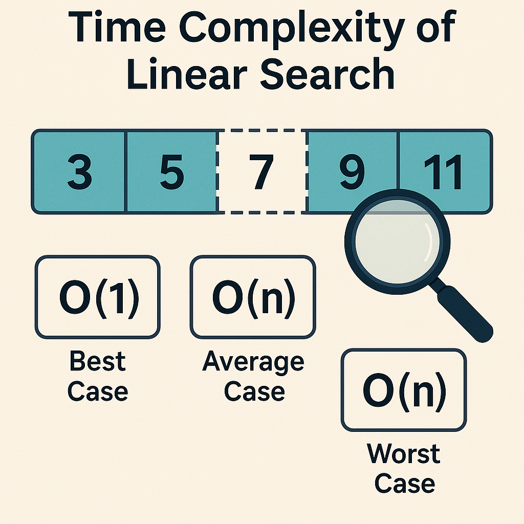
• Best Case: What's the luckiest we can get? The target element is the very first one in the array (arr[0]). The loop runs only once, performs one comparison, and returns immediately. The time taken is constant, regardless of the array's size.

  • Complexity: O(1)

• Worst Case: What's the unluckiest scenario? There are two possibilities: the target is the very last element, or it's not in the array at all. In both situations, the algorithm must iterate through the entire array, making n comparisons.

  • Complexity: O(n)

• Average Case: Assuming the target is in the array and every position is equally likely, we would expect to find the element somewhere in the middle. On average, we would search through n/2 elements. Since we drop constants in Big O notation, this simplifies to linear time.

  • Complexity: O(n)

These images provide a great visual summary of the analysis for linear search.

To solidify this, let's read the section from GeeksforGeeks that details this exact example.

Cases vs. Asymptotic Notations: A Crucial Clarification

A very common point of confusion is mapping cases directly to notations. Many people mistakenly believe:

• Big O is for the worst case.
• Big Omega (Ω) is for the best case.
• Big Theta (Θ) is for the average case.

This is incorrect.

Asymptotic notations (O, Ω, Θ) are mathematical tools used to describe the growth rate of functions. Best, worst, and average cases are types of analysis that produce these functions. You can use any notation to describe the result of any case analysis.

For linear search:

• The best-case running time is 1. We can say it's O(1), Ω(1), and Θ(1).
• The worst-case running time is n. We can say it's O(n), Ω(n), and Θ(n).

The renowned instructor Abdul Bari has an excellent explanation that clarifies this distinction perfectly.

The Primacy of Worst-Case Analysis

In professional software development, while all three cases provide insight, the worst-case analysis (Big O) is given the most weight. Your experience designing backend systems and APIs will make the reasons for this immediately apparent. You must design for reliability, scalability, and predictable performance, even under maximum stress.

Case Study 2: When Cases Have Different Complexities

Linear search showed us a O(1) best case and a O(n) worst case. Let's look at another example where the difference is even more stark. Consider this simple algorithm:

public int specialArraySum(int[] arr) {
    int n = arr.length;

    // Best-case scenario
    if (n % 2 == 0) {
        return 0; // Constant time operation
    }

    // Worst-case scenario
    int sum = 0;
    for (int num : arr) {
        sum += num;
    }
    return sum; // Linear time operation
}

This function behaves differently based on a property of the input: the length of the array.

• Best Case: If the input array has an even length, the function checks n % 2 == 0, finds it true, and returns 0 immediately. This is a constant time operation.

  • Complexity: O(1)

• Worst Case: If the input array has an odd length, the function performs the check, finds it false, and then proceeds to loop through all n elements to calculate their sum. This is a linear time operation.

  • Complexity: O(n)

• Average Case: If we assume that even and odd length arrays are equally likely inputs, then half the time the algorithm is O(1) and half the time it is O(n). The O(n) term dominates the average, so we consider the average case to be linear.

  • Complexity: O(n)

This contrived example clearly illustrates how an algorithm's complexity can fundamentally change based on the characteristics of the input. You can read the original analysis of this example in the GeeksforGeeks article.

Conclusion

This lesson completes our foundational module on complexity analysis. You've moved from a general understanding of Big O to a more sophisticated view that accounts for performance variations based on specific input data.

Key Takeaways:

• An algorithm's performance is not fixed; it varies with the input.
• Best-case analysis gives an optimistic lower bound (O(1) for linear search).
• Worst-case analysis provides a pessimistic upper bound and a performance guarantee (O(n) for linear search). It is the most critical for designing reliable systems.
• Average-case analysis offers a realistic prediction but can be complex to calculate (O(n) for linear search).
• Cases (best, worst, average) are types of analysis, while notations (O, Ω, Θ) are the mathematical language used to express the results of that analysis.

You now possess the essential theoretical framework to analyze and compare algorithms. In our next module, we will put this theory into practice as we begin our journey into data structures, starting with the most fundamental of all: arrays. We will explore common array operations and powerful problem-solving patterns like the two-pointer and sliding window techniques, analyzing the complexity of each along the way.