Introduction
In our last lesson, we mastered Gauss-Jordan elimination, a powerful algorithm for transforming an augmented matrix into its unique reduced row echelon form (RREF). For systems with a single, unique solution, this process made the answer immediately apparent. However, not all systems of linear equations behave so neatly.
This lesson addresses the remaining possibilities. We will explore how to use the row echelon form of an augmented matrix to determine precisely whether a system has no solution, a unique solution, or infinitely many solutions. By the end of our session, you'll be able to diagnose the nature of any linear system just by examining the positions of the pivots in its row-reduced form.
Geometrically, for a simple system of two equations in two variables, these three outcomes are easy to visualize.
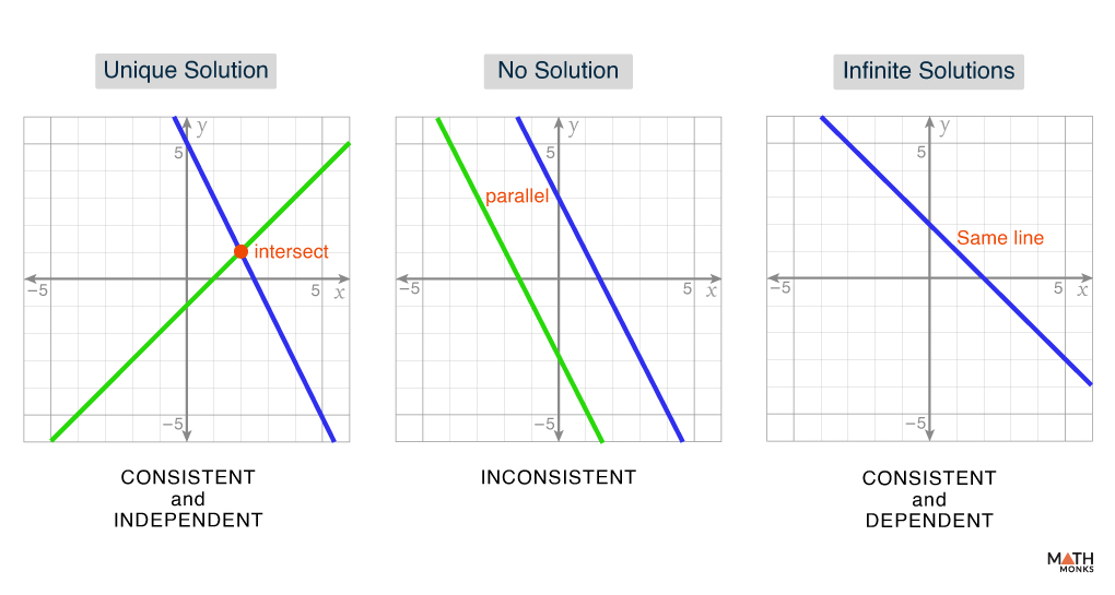
Our goal is to develop a systematic algebraic method that works for any number of equations and variables.
The Anatomy of a Solution Set
After you perform Gaussian or Gauss-Jordan elimination to bring an augmented matrix into row echelon form (REF) or reduced row echelon form (RREF), the number of solutions to the system is revealed by the placement of the pivot entries.
There are fundamentally three scenarios, which are neatly summarized in the following document.
This reading from a Georgia Tech course outlines the "trichotomy"—the three distinct possibilities for the solution set of a linear system, based on the structure of its reduced row echelon form.
Please read the section titled "Trichotomy". Focus on understanding the connection between the location of pivot columns and the three outcomes: zero, one, or infinite solutions.
As the reading explains, the first crucial question is whether the system is consistent (has at least one solution) or inconsistent (has no solution). This single distinction is our starting point.
Case 1: No Solution (Inconsistent Systems)
An inconsistent system is one that contains a contradiction. In the context of row reduction, this contradiction appears in a very specific way.
Consider a row in your augmented matrix (in REF or RREF) that looks like this:
where is a non-zero number. If we translate this row back into an equation, we get:
This simplifies to the statement , which is a clear contradiction. Since this equation can never be true, the entire system has no solution.
This situation occurs if and only if the augmented column is a pivot column. In other words, after row reduction, there is a pivot in the rightmost column of the augmented matrix.
The following video provides a clear explanation of this case.
Zero, One, or Infinitely Many Solutions? [Passing Linear Algebra]
This video, "Zero, One, or Infinitely Many Solutions?", explains how to identify each solution type from a row-reduced matrix.
Watch the segment explaining the "no solution" case. The presenter shows how a pivot in the augmented column leads to a nonsensical equation like 0 = 3, indicating an inconsistent system.
Case 2: At Least One Solution (Consistent Systems)
If a system is not inconsistent, it must be consistent, meaning it has at least one solution. This is the case when, after row reduction, there is no pivot in the augmented column.
Once we know a system is consistent, we then need to determine if it has exactly one solution or infinitely many. This distinction depends on the concept of free variables.
Free Variables
A variable is called a free variable if its corresponding column in the coefficient matrix (the part to the left of the augmentation line) is not a pivot column. This means that after row reduction, the column for that variable does not contain a pivot.
A free variable is "free" because its value is not fixed by one of the equations. We can choose any value for it, and the other variables will adjust accordingly. The presence of even one free variable opens the door to an infinite number of solutions.
Let's explore this idea further with a reading.
This document section formally defines free variables and shows how they lead to infinitely many solutions, which are expressed using a "parametric form".
In the document, start at the beginning of Section 1.3 to see how a column without a pivot leads to a free variable. Continue reading to understand how the solution set is expressed in parametric form, where the pivot variables are written in terms of the free variables.
Now we can distinguish between our final two cases.
Sub-Case 2a: A Unique Solution
A consistent system has a unique solution if and only if there are no free variables.
This means that every column in the coefficient matrix must be a pivot column. When you look at the RREF of such a system, it will typically look something like the identity matrix on the left, with the solution vector on the right:
This corresponds to the equations , , and , which is a single, unique solution.
Watch this segment of the video for a quick summary of this case.
Zero, One, or Infinitely Many Solutions? [Passing Linear Algebra]
Continuing with the same video.
Watch the explanation for the "one solution" case. The key takeaway is that the system must be consistent and have no free variables.
Sub-Case 2b: Infinitely Many Solutions
A consistent system has infinitely many solutions if and only if there is at least one free variable.
If a column in the coefficient matrix lacks a pivot, the corresponding variable is free. Since that variable can be any real number, and the other (pivot) variables can be expressed in terms of it, there is an infinite family of solutions. As you saw in the reading, we describe this infinite set using a parametric form.
For example, if a row-reduced system yields:
Here, the pivot columns are 1 and 2, so and are pivot variables. Column 3 has no pivot, so is a free variable. We express the solution by solving for the pivot variables in terms of the free one:
For any choice of , we get a valid solution.
The video explains this scenario as well.
Zero, One, or Infinitely Many Solutions? [Passing Linear Algebra]
One last clip from this video.
Watch the segment on infinitely many solutions. Notice how the presence of a free variable in a consistent system requires the solution to be written in parametric form.
Putting It All Together: A Decision Process
You can now use a simple process to determine the number of solutions for any system:
- Row Reduce: Transform the augmented matrix into row echelon form (REF).
- Check for Consistency: Is there a row of the form where ?
- Yes: The system is inconsistent. It has zero solutions.
- No: The system is consistent. Proceed to the next step.
- Check for Free Variables: Are there any columns in the coefficient matrix that do not contain a pivot?
- No: There are no free variables. The system has a unique solution.
- Yes: There is at least one free variable. The system has infinitely many solutions.
To see this process in action, watch the presenter in the video apply these rules to five different matrices. Try to pause before each example and decide on the solution type yourself.
Zero, One, or Infinitely Many Solutions? [Passing Linear Algebra]
This is the final segment of the video "Zero, One, or Infinitely Many Solutions?".
Watch the worked examples from this point to the end. For each of the five matrices, identify the pivots and use the decision process to determine if there are zero, one, or infinitely many solutions.
Conclusion
In this lesson, we completed our exploration of solving systems of linear equations. We moved beyond finding a single solution and learned to use the structure of a matrix in row echelon form to classify the entire solution set.
Here are the key takeaways:
- A linear system can have only zero, one, or infinitely many solutions.
- A system has zero solutions (is inconsistent) if and only if its row echelon form has a pivot in the augmented column, leading to a contradiction like .
- A system is consistent if it has no pivot in the augmented column.
- A consistent system has a unique solution if every column in the coefficient matrix is a pivot column (no free variables).
- A consistent system has infinitely many solutions if there is at least one non-pivot column in the coefficient matrix (at least one free variable). The solution is then described using a parametric form.
So far, we have solved the equation using row reduction. In the next module, we will begin exploring the properties of the matrix itself, starting with the concept of the matrix inverse. This will eventually provide us with an entirely new, and in some cases more elegant, way to solve for when a unique solution exists.