Factored Permanent Loads for Steel Bridges

1. Identifying Permanent Loads: DC and DW

Permanent loads are those that are expected to be present on the bridge for its entire design life. AASHTO LRFD categorizes them into two main groups to reflect different levels of uncertainty in their magnitude.

• DC: Dead Load of Components and Attachments: This includes the weight of all structural and non-structural elements that are a permanent part of the bridge. As a designer, you have significant control over these quantities.
• DW: Dead Load of Wearing Surfaces and Utilities: This includes the weight of components that are also permanent but may be subject to more variation over the life of the structure, such as future asphalt overlays.

The image below shows a typical steel I-girder bridge cross-section. Before we proceed, take a moment to identify which elements you would classify as DC and which as DW.

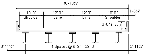
In this cross-section, the DC components include:

• The steel I-girders themselves.
• Any cross-frames or diaphragms connecting the girders (not visible in this 2D view).
• The cast-in-place concrete deck and the haunch area above the steel flanges.
• The concrete parapets (barriers) on the shoulders.

The DW component is the future wearing surface. This is an allowance for future asphalt overlays that will be placed on the deck. Its weight is specified by the owner, often as a pressure (e.g., psf or kPa).

Because the DC components are well-defined by the design drawings and material specifications, their load factor is lower. The DW loads, particularly the future wearing surface, are less certain—its thickness can vary significantly over the life of the bridge due to multiple paving operations. Consequently, AASHTO assigns it a higher load factor. For the primary Strength I load combination, the factors are:

• ${\gamma }_{DC}=1.25$
• ${\gamma }_{DW}=1.50$

2. Calculating Nominal Permanent Loads

The next step is to calculate the nominal (unfactored) weight of these components, typically expressed as a distributed load in units of kips per linear foot (klf) or kN/m. This involves using standard material unit weights and the geometric properties of the cross-section.

We will walk through a practical example from an FHWA design guide for strengthening a plate girder bridge. While the context is strengthening, the initial steps involve a clear and detailed calculation of the existing dead loads, making it an excellent learning resource.

As you can see from the example, the process is systematic:

1. Calculate the weight of each individual component per unit length of the bridge.
2. For components like parapets or wearing surfaces that are applied over a certain width, their total weight is distributed among the supporting girders. The example shows this for a multi-girder bridge; for our target two-girder tub system, the distribution would be determined based on a tributary width or a more refined analysis.
3. Sum the individual component weights into the appropriate AASHTO categories: DC and DW. In the example, all components except the overlay are grouped into uDC1.

3. Assembling Factored Loads for the Strength I Limit State

Once the nominal dead loads, $w_{DC}$ and $w_{DW}$, are determined, we can assemble the factored load for the Strength I limit state. Let's revisit the formula from the curved box girder design example, which we will use throughout this course.

The permanent load portion of the Strength I combination is:

Using the numerical values from the LINK design example:

• $w_{DC}=uDC1=1.369\text{ klf}$
• $w_{DW}=uDW=0.197\text{ klf}$

Assuming a load modifier $\eta =1.0$ for this example, the factored permanent load per girder would be:

This factored uniform load is then applied to the analytical model of the bridge to calculate the factored design moments and shears. The tables in the LINK example show this final output.

4. Application to a Trapezoidal Tub Girder

The principles remain identical for the trapezoidal tub girders that are the focus of this course. The components are largely the same: steel tub weight, concrete deck, haunches, stay-in-place forms, parapets, and a wearing surface. The primary difference is the geometry used for calculating the weights and section properties.

The design example for a curved box girder shows how these loads are defined and applied in a more complex analysis.

This demonstrates that regardless of the structural system's complexity or the analysis method used, the fundamental first step is always the careful calculation and categorization of permanent loads based on AASHTO DC and DW definitions.

Conclusion

In this lesson, we have moved from the abstract LRFD equation to its first practical application. We have defined the AASHTO permanent load categories, calculated their nominal values based on a worked example, and assembled them using the appropriate load factors for the Strength I limit state.

Key Takeaways:

• Permanent loads in AASHTO are divided into DC (Components) and DW (Wearing Surfaces) to reflect different levels of uncertainty.
• The standard load factors for the Strength I limit state are ${\gamma }_{DC}=1.25$ and ${\gamma }_{DW}=1.50$.
• The calculation process involves determining the weight per unit length of each component (steel, deck, barriers, etc.) and summing them into the DC and DW categories.
• These factored loads are then used in the structural analysis to determine the design moments, shears, and other force effects.

Now that we have a solid grasp of how to handle permanent loads, we are ready to tackle the more dynamic and statistically complex world of transient loads. In our next lesson, we will dive into the AASHTO HL-93 vehicular live load model, including the dynamic load allowance (IM) and multiple presence factors.