Diagonalizing the Tight-Binding Hamiltonian

Welcome to the second lesson on the tight-binding model. Last time, we carefully constructed the model's Hamiltonian in the real-space basis, capturing the physics of electrons hopping between adjacent lattice sites. We arrived at the expression:

H^_{TB} = - t ⟨ i, j ⟩, σ \sum (c_{iσ}^{†} c_{j σ} + c_{j σ}^{†} c_{iσ})

You'll notice that this Hamiltonian contains terms like $c_{iσ}^{†} c_{j σ}$ where $i \neq = j$ . These terms mix different site basis states, meaning the Hamiltonian is not diagonal in this basis. Our goal in this lesson is to find a basis that does diagonalize $H^_{TB}$ . The eigenvalues in this new basis will give us the energy spectrum of the system, a crucial property known as the band structure.

Because the crystal lattice is periodic, the Hamiltonian possesses translational symmetry. This is a strong hint that the eigenstates will be labeled by a crystal momentum wavevector, $k$ , as dictated by Bloch's theorem. The mathematical tool for moving from a real-space representation to a momentum-space representation is the Fourier transform. This process is analogous to how one transforms a system of classically coupled oscillators into a set of uncoupled normal modes, each with its own characteristic frequency. Here, we will decouple the electron hopping between sites into independent electron modes, each with a specific momentum $k$ and energy $E (k)$ .

From Site to Momentum Operators

Our first step is to define a new set of fermionic operators that create and annihilate electrons in states of definite momentum, rather than definite position. These are defined as the discrete Fourier transforms of the real-space operators.

Tight-Binding Model in the Second Quantization Formalism

This document provides a concise mathematical guide to transforming the tight-binding model. We will first focus on the definitions of the operators.

In section 1.1, "Representations and bases," please read from the beginning to the end of the section. Focus on the relationship between operators in different bases and, specifically, the definitions given in Eqs. (13) and (14). These equations define the forward and inverse Fourier transforms connecting the real-space operators (c_j, c^\dagger_j) and momentum-space operators (c_k, c^\dagger_k).

As the reading shows, the transformations are:

c_{j σ} = \frac{1}{N} k \sum e^{ik \cdot r_{j}} c_{k σ} and c_{j σ}^{†} = \frac{1}{N} k \sum e^{- ik \cdot r_{j}} c_{k σ}^{†}

And the inverse transforms are:

c_{k σ} = \frac{1}{N} j \sum e^{- ik \cdot r_{j}} c_{j σ} and c_{k σ}^{†} = \frac{1}{N} j \sum e^{ik \cdot r_{j}} c_{j σ}^{†}

Here, $N$ is the number of lattice sites, $r_{j}$ is the position vector of site $j$ , and the sum over $k$ is over all allowed wavevectors in the first Brillouin zone. It can be verified that the momentum-space operators $c_{k σ}$ and $c_{k σ}^{†}$ also obey the canonical fermionic anticommutation relations, e.g., ${c_{k σ}, c_{k^{'} σ^{'}}^{†}} = δ_{k k^{'}} δ_{σ σ^{'}}$ .

Diagonalizing the Hamiltonian

Now we can perform the main task: substituting these transformations into our tight-binding Hamiltonian to express it in the momentum basis. The algebra involves combining the exponential terms and using a key identity about sums over lattice vectors.

The following reading details this exact procedure.

Tight-Binding Model in the Second Quantization Formalism

We will now continue with the same document to see how these operator transformations diagonalize the Hamiltonian.

Read section 2.2, "Momentum-space representation." Follow the derivation closely, starting from the rewriting of the nearest-neighbor sum in Eq. (29). The crucial step is the substitution of the momentum-space operators and the use of the lattice sum identity (Eq. 16) to simplify the expression. Your goal is to understand how this leads to the diagonal form in Eqs. (30) and (31).

The derivation shows that after substituting the Fourier-transformed operators, the Hamiltonian becomes:

H^_{TB} = k, σ \sum E (k) c_{k σ}^{†} c_{k σ}

where the energy dispersion relation, or band structure, is given by:

E (k) = - t δ \sum cos (k \cdot δ)

Here, the sum is over all vectors $δ$ connecting a site to its nearest neighbors.

The Hamiltonian is now diagonal! Each term $c_{k σ}^{†} c_{k σ}$ is simply the number operator for electrons with momentum $k$ and spin $σ$ . There are no terms that mix different momentum states. The problem has been decoupled into a set of independent single-particle energy levels $E (k)$ .

For a spoken explanation of this same derivation, you can watch the following segment from Professor James Freericks' lecture.

lecture38 The Hubbard Model

This video provides a lecture-style walkthrough of the Fourier transformation of the tight-binding kinetic energy term.

Watch the segment from here. The lecturer defines the momentum-space operators (which he calls a_k) and substitutes them into the hopping Hamiltonian. Pay attention to how the sum over lattice sites results in a delta function in momentum, diagonalizing the kinetic term. He arrives at the same dispersion relation involving the sum of cosines.

The Band Structure of a 1D Chain

Let's make this concrete by applying the general result to a one-dimensional chain of atoms with lattice spacing $a$ . For any given site, the nearest neighbors are at positions $+ δ$ and $- δ$ , where $δ = a x^$ . The wavevector $k$ is a scalar in 1D.

The sum over nearest-neighbor vectors $δ$ has two terms:

E (k) = - t (cos (k \cdot (a x^)) + cos (k \cdot (- a x^)))

Since $cos (- x) = cos (x)$ , this simplifies beautifully to:

E (k) = - 2 t cos (k a)

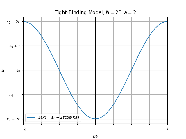
This is the famous energy band for the 1D tight-binding model. The allowed values of $k$ lie in the first Brillouin zone, which for a 1D chain is $k \in [- π / a, π / a]$ .

Let's analyze this result:

The energy is a periodic function of $k$ with period $2 π / a$ .
The minimum energy is at $k = 0$ , where $E (0) = - 2 t$ . This corresponds to a state where all site wavefunctions add constructively, maximizing delocalization and kinetic energy saving.
The maximum energy is at the Brillouin zone edge, $k = \pm π / a$ , where $E (\pm π / a) = + 2 t$ . This corresponds to a state where adjacent site wavefunctions have opposite signs, which is energetically unfavorable.
The bandwidth, the total range of energies, is $E_{ma x} - E_{min} = 4 t$ . This confirms our intuition: the larger the hopping parameter $t$ , the wider the band and the more itinerant the electrons.

The plot below shows this cosine band. Sometimes an on-site energy $ϵ_{0}$ is included, which simply shifts the entire band up or down, giving $E (k) = ϵ_{0} - 2 t cos (k a)$ .

The analytical band structure for a 1D tight-binding model. The energy E is plotted against the dimensionless wavevector ka, showing the characteristic cosine dispersion.

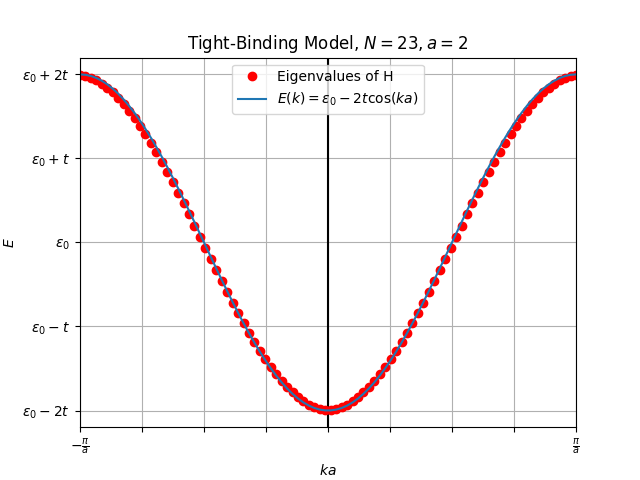
Your experience with numerical methods will appreciate this next point. What we just did analytically is equivalent to constructing the real-space Hamiltonian as a large $N \times N$ matrix and numerically finding its eigenvalues. The Fourier transform is an elegant analytical shortcut to the same result for a periodic system.

The following image illustrates this perfectly. The red dots are the eigenvalues calculated numerically for a finite chain with $N = 23$ sites. The blue line is our analytical formula. The agreement is exact.

A comparison between the numerically computed eigenvalues of the real-space Hamiltonian for a finite chain (N=23) and the analytical dispersion relation derived via Fourier transform. The perfect match validates the analytical method.

Conclusion

In this lesson, we have successfully diagonalized the tight-binding Hamiltonian and found its energy spectrum. This is a pivotal result that forms the basis for understanding electronic properties of solids.

The key takeaways are:

Diagonalization via Fourier Transform: The translational symmetry of the lattice allows the tight-binding Hamiltonian to be diagonalized by transforming the creation and annihilation operators from the real-space (site) basis to the momentum basis.
The Band Structure $E (k)$ : The eigenvalues of the Hamiltonian are the single-particle energies $E (k)$ , which form a continuous band. The shape of this band, or dispersion relation, is determined by the lattice geometry and is given by $E (k) = - t \sum_{δ} cos (k \cdot δ)$ .
1D Chain: For a 1D chain, the band structure is a simple cosine band, $E (k) = - 2 t cos (k a)$ , with a bandwidth of $4 t$ .

We now have a complete picture of the single-particle energy levels in a non-interacting system. In the next lesson, we will use this result to construct the many-body ground state of the system by filling these energy levels with electrons, and we will explore how properties like electron density are calculated.

Recommended resources

From Site to Momentum Operators

Diagonalizing the Hamiltonian

The Band Structure of a 1D Chain

Conclusion