Calculus Applications: Integration and Differentiation

Welcome back to our course on Probability. In our previous lesson, we established a foundation for working with discrete series of numbers using summation and product notation. These tools are perfect for situations where outcomes are countable, like the results of a dice roll. However, many real-world phenomena are not countable but continuous—think of measurements like time, length, or temperature.

In this lesson, we will pivot from the discrete world of sums to the continuous world of curves and areas. We'll achieve this by reviewing and applying key concepts from single-variable calculus. You will see how differentiation and integration are not just abstract mathematical tools but are in fact the natural language for describing and solving problems in continuous probability. By the end of this lesson, you'll be able to use these calculus techniques to work with one of the most important concepts in this field: the probability density function.

A Refresher on Differentiation

Before we dive into probability applications, let's refresh our memory on the fundamental rules of differentiation. The derivative of a function gives us its instantaneous rate of change, or the slope of the tangent line at any point. A solid command of these rules is essential.

The following video provides an excellent and concise review of the main differentiation rules you'll need. As you watch, focus not just on the formulas themselves, but on recognizing when to apply each rule.

Review of all Derivative Rules | Calculus | jensenmath

This video from JensenMath offers a clear and example-driven review of essential derivative rules.

Please watch the following segments. The goal is to reactivate your knowledge of these core techniques. Power and Constant Multiple Rules: Watch the first example from the beginning to see the most fundamental rule in action. Product Rule: Next, review the explanation and example for differentiating a product of two functions from this section. Quotient Rule: Watch the segment from this point on the quotient rule, used for functions that are fractions. Chain Rule: Finally, watch the introduction to the chain rule for composite functions, from this segment.

These rules—especially the power rule and chain rule—will appear frequently as we move forward.

From Discrete Sums to Continuous Integrals

In the last lesson, we worked with sums. For continuous phenomena, integration takes the place of summation. Let's introduce a central concept where this transition becomes clear: the continuous random variable.

While a discrete random variable can only take on specific, separate values (e.g., the numbers 1 through 6 on a die), a continuous random variable can take on any value within a given range (e.g., the exact height of a person or the time you wait for a bus).

We describe the probabilities associated with a continuous random variable using a Probability Density Function (PDF), denoted as $f (x)$ .

Calculus II - Probability

This page from Paul's Online Math Notes provides a concise introduction to the role of calculus in probability.

Read the introductory text, starting from the beginning and ending just before Example 1. Focus on the definition of a continuous random variable and the two crucial conditions that a probability density function must satisfy.

As you just read, a function $f (x)$ is a valid PDF if it meets two conditions:

It is non-negative: $f (x) \geq 0$ for all $x$ . This makes sense, as probability cannot be negative.
The total area under its curve is 1: $\int_{- \infty}^{\infty} f (x) d x = 1$ . This is the continuous equivalent of saying that the sum of all possible probabilities must equal 1.

Calculating Probabilities with Integration

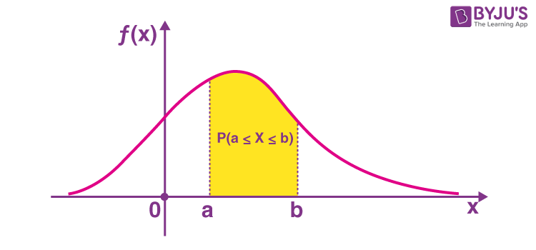
The most important application of the PDF is calculating the probability that a random variable $X$ falls within a certain interval, say between $a$ and $b$ . This probability is simply the area under the PDF curve from $a$ to $b$ . We find this area using a definite integral.

P (a \leq X \leq b) = \int_{a}^{b} f (x) d x

The image below provides a clear visualization of this concept. The shaded area under the curve $f (x)$ from $a$ to $b$ represents the probability that our random variable $X$ will take a value in that range.

The probability that a continuous random variable X falls between values 'a' and 'b' is the definite integral of its probability density function f(x) from 'a' to 'b', represented by the area of the shaded region.

Let's see this in action. The following resources walk through complete examples of verifying a PDF and using it to calculate probabilities.

Calculus II - Probability

Let's continue with the Paul's Online Math Notes page.

Carefully study Example 1 in its entirety. It shows you how to: Verify a function is a PDF by showing its integral over its domain equals 1. Calculate the probability that X falls within a specific range, P(1 \le X \le 4), by integrating over that range. Calculate the probability over a tail-end range, P(X \ge 6).

To reinforce this process, let's watch a video that works through a similar problem.

Probability Density Functions

This video by The Organic Chemistry Tutor provides another excellent, step-by-step example.

Watch the first part of the video, which covers a problem very similar to the one you just read about. First, see how to verify a PDF using integration. Then, watch how to calculate probabilities for different intervals like P(X > 4) and P(1 < X < 3). Notice that for continuous variables, P(X > 4) is the same as P(X \ge 4). The probability of X being exactly equal to any single point is zero, which is a key difference from discrete variables.

Finding the Mean (Expected Value)

Just as we can calculate the mean, or expected value, of a discrete random variable using summation, we can find the mean of a continuous random variable using integration. The mean, denoted by $μ$ , represents the long-term average value of the random variable.

The formula is a continuous analogue of a weighted average: each possible value $x$ is weighted by its probability density $f (x)$ .

μ = \int_{- \infty}^{\infty} x \cdot f (x) d x

The examples you have already reviewed demonstrate this concept.

Calculus II - Probability

Let's return one last time to the Paul's Online Math Notes page.

First, read the brief section that introduces the formula for the mean. Then, review Example 2, particularly part (c), which shows how to calculate the mean for an exponential density function. This example involves an improper integral, which is common when dealing with variables that have no upper bound (like time).

Finding the PDF from the Cumulative Distribution Function (CDF)

So far, we have used integration on the PDF to find area (probability). Now, let's use the other side of calculus: differentiation.

First, we need to define the Cumulative Distribution Function (CDF), $F_{X} (x)$ , which gives the probability that the random variable $X$ is less than or equal to some value $x$ .

F_{X} (x) = P (X \leq x) = \int_{- \infty}^{x} f_{X} (u) d u

The Fundamental Theorem of Calculus tells us that differentiation and integration are inverse operations. This leads to a powerful and elegant relationship: the PDF is the derivative of the CDF.

f_{X} (x) = \frac{d}{d x} F_{X} (x) = F_{X}^{'} (x)

This gives us a direct application for the differentiation rules we reviewed at the start of the lesson. If you know a variable's CDF, you can find its PDF by simply taking the derivative.

Probability Density Function | PDF

This page from ProbabilityCourse.com explains the relationship between the PDF and CDF.

Read the section titled Probability Density Function (PDF). Focus on the derivation that shows the PDF is the derivative of the CDF, summarized in the equation f_X(x) = F'_X(x). Also, look at the example that follows, where the PDF of a Uniform random variable is found by differentiating its CDF.

Conclusion

In this lesson, you've seen how single-variable calculus is not just a prerequisite for studying probability, but an active and essential part of it. We've bridged the gap between the discrete sums of our last lesson and the continuous integrals needed for many real-world models.

Here are the key takeaways:

Continuous random variables are described by a Probability Density Function (PDF), $f (x)$ , where the total area under the curve is 1.
Integration is the tool used to calculate probabilities. The probability $P (a \leq X \leq b)$ is the definite integral of the PDF from $a$ to $b$ .
Integration is also used to find the mean (expected value) of a continuous random variable.
Differentiation provides the link from the Cumulative Distribution Function (CDF) back to the PDF, as $f_{X} (x) = F_{X}^{'} (x)$ .

In our next lesson, we will extend our calculus toolkit further by reviewing double integrals. This will prepare us to analyze scenarios involving multiple random variables, a cornerstone of more advanced probability theory.

Recommended resources

A Refresher on Differentiation

From Discrete Sums to Continuous Integrals

Calculating Probabilities with Integration

Finding the Mean (Expected Value)

Finding the PDF from the Cumulative Distribution Function (CDF)

Conclusion