Welcome back. In our last lesson, we introduced the key metrics for assessing how well a single model fits the data: Residual Standard Error (RSE) and R-squared. We also highlighted a critical flaw with R-squared—it misleadingly increases as you add more variables.
This lesson is dedicated to mastering the solution: Adjusted R-squared. Your ability to use this metric is not just a theoretical point; it's one of the most common tasks on a practical exam, where you'll be asked to compare several competing models and justify your choice. We will focus entirely on the purpose of Adjusted R-squared and how to use it to make a clear, defensible decision.
The Problem with R-squared: The Overfitting Trap
Let's start by reinforcing a concept we touched on previously, as it's a very common exam trap. The standard R-squared metric, , measures the proportion of variance in the response variable that is explained by your predictors. However, it has a major weakness: it will always increase (or at best, stay the same) every time you add a new predictor to the model. This happens even if the new variable is completely irrelevant and adds no real explanatory power.
Chasing a high by blindly adding variables leads to overfitting. An overfit model is one that is too complex; it has learned the "noise" and random quirks in your specific sample data rather than the true underlying relationship. While it might look great on the data it was trained on, it will perform poorly when making predictions on new, unseen data.
The article "How to Interpret Adjusted R-Squared" by Jim Frost clearly explains this issue.
How to Interpret Adjusted R-Squared and Predicted R ...
This article directly addresses the problems with standard R-squared that make Adjusted R-squared necessary.
Read the section titled "Some Problems with R-squared". Focus on the two key problems the author identifies: the automatic increase with more variables and the danger of overfitting.
The Solution: Adjusted R-squared's Penalty System
Adjusted R-squared is a modified version of R-squared that is specifically designed to address this problem. It "adjusts" the R-squared value by adding a penalty for each additional predictor in the model.
Here’s the core logic you need to understand for your exam:
- If you add a useful predictor to the model (one that explains a significant amount of new variance), the increase in R-squared will outweigh the penalty. As a result, Adjusted R-squared will increase.
- If you add a useless predictor to the model (one that is just noise), the small, automatic increase in R-squared will not be enough to overcome the penalty. As a result, Adjusted R-squared will decrease.
This video provides an excellent intuitive explanation of this penalty mechanism.
Adjusted R squared vs. R Squared For Beginners | By Dr. Ry @Stemplicity
This video from Prof. Ryan Ahmed uses a simple, practical example to show why R-squared is flawed and how Adjusted R-squared provides a solution.
Watch the segment from this video clip. Pay close attention to the example where a useless variable ("education of worker") is added to a model predicting ice cream revenue. Notice how the presenter explains that R-squared will go up, but this is misleading, and Adjusted R-squared is designed to correct for this.
Because of this penalty system, Adjusted R-squared is the appropriate metric for comparing models that have different numbers of predictor variables.
Putting it into Practice: Comparing Models
For your exam, you will almost certainly be presented with the output of several models and asked to choose the "best" one. The primary tool for this is Adjusted R-squared.
What to Look For:
Look at a "Best Subsets" or similar model comparison output. You will see a list of models with different combinations of predictors. For each model, you'll see R-squared, Adjusted R-squared, and other metrics.
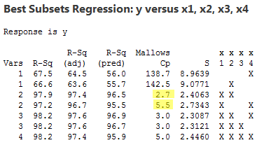
Let's analyze the output in the image above:
-
Observe R-squared: Look at the
R-Sqcolumn. As the number of variables (Vars) increases from 1 to 4, the R-squared value consistently goes up, from a max of 67.5% for one variable to 98.2% for four variables. This demonstrates the exact problem we discussed. If you only looked at R-squared, you would always choose the most complex model. -
Analyze Adjusted R-squared: Now look at the
R-Sq(adj)column. This tells a different story.- The best 1-variable model has an Adjusted R-squared of 64.5%.
- Adding a second variable (
x1,x2) provides a huge jump to 97.4%. This was clearly a very useful addition. - Adding a third variable (
x1,x2,x3) nudges the Adjusted R-squared up slightly to 97.6%. This is the highest value in the table. - Adding the fourth variable causes the Adjusted R-squared to drop to 97.4%. This is the penalty in action! The fourth variable did not add enough explanatory power to justify its inclusion.
How to Interpret (Exam-Style Sentence):
When asked to choose the best model from this output, your reasoning should be as follows:
The model with three predictors (x1, x2, and x3) is the preferred model. It has the highest Adjusted R-squared (97.6%), indicating it provides the best fit to the data after penalizing for model complexity. Including the fourth predictor is not justified, as it causes the Adjusted R-squared to decrease.
Practice Drill
You are comparing three different models to predict the quarterly sales of a company (in thousands of dollars).
- Model 1: Predicts
SalesusingAdvertising Spend.- R-squared = 0.55
- Adjusted R-squared = 0.54
- Model 2: Predicts
SalesusingAdvertising SpendandNumber of Sales Reps.- R-squared = 0.62
- Adjusted R-squared = 0.60
- Model 3: Predicts
SalesusingAdvertising Spend,Number of Sales Reps, andAverage Competitor Price.- R-squared = 0.63
- Adjusted R-squared = 0.59
Your Task:
- A colleague argues for Model 3 because it has the highest R-squared (0.63). In one sentence, explain why this reasoning is flawed.
- Which model is the best choice according to the principle of Adjusted R-squared?
- Write a 2-line, exam-style justification for your choice.
Solution
-
Flawed Reasoning: This reasoning is flawed because R-squared will always increase when adding predictors, even useless ones, and should not be used to compare models with different numbers of variables.
-
Best Model: Model 2 is the best choice.
-
Exam-Style Justification:
Model 2 is the preferred model as it possesses the highest Adjusted R-squared (0.60). This indicates that it offers the optimal balance between explanatory power and model simplicity, as adding the third predictor in Model 3 caused the Adjusted R-squared to decrease.
Conclusion
You have now mastered a crucial skill for your practical exam: using Adjusted R-squared to compare and select regression models. Remember this simple rule: when comparing models with different numbers of predictors, ignore R-squared and focus on Adjusted R-squared.
Key Takeaways for Your Exam:
- The Trap: R-squared always increases with more variables, which can lead to overfitting. Do not use it to compare models with different numbers of predictors.
- The Tool: Adjusted R-squared penalizes the model for complexity, making it the correct tool for model comparison.
- The Rule: When comparing models, choose the one with the highest Adjusted R-squared (while also considering the RSE, as learned in the last lesson).
In our next lesson, we will dive into the ANOVA table. This introduces the F-statistic, which gives us a formal statistical test to determine if our model, as a whole, is statistically significant. This complements the descriptive fit statistics we've just covered by adding a layer of inferential testing.