Optimizing Queries with Logical Transformations

The Philosophy of Rule-Based Optimization

Before diving into specific rules, let's establish the overall philosophy. The optimizer takes an initial logical plan (represented as a tree of relational algebra operators) and applies a series of equivalence rules to transform it. An equivalence rule allows us to replace one expression with another that produces the exact same result.

For example, σ_{p1 AND p2}(R) is equivalent to σ_{p1}(σ_{p2}(R)).

This process is often called heuristic optimization or rule-based optimization because the rules are applied based on heuristics that are almost always beneficial, without yet needing to calculate the precise "cost" of each alternative. The primary goal is to reduce the amount of data that flows between operators as early as possible.

To see how a database system approaches this, let's get an overview of the process.

As you saw, a few simple rewrites can dramatically change the structure of the query plan, making it look much more sensible. Now, let's explore the most important of these rules in more detail.

Predicate Pushdown: The Golden Rule

If there's one transformation to remember, it's predicate pushdown. The principle is simple: perform selections (filters) as early as possible. By filtering out rows you don't need before they enter expensive operations like joins, you can drastically reduce the amount of work the database has to do.

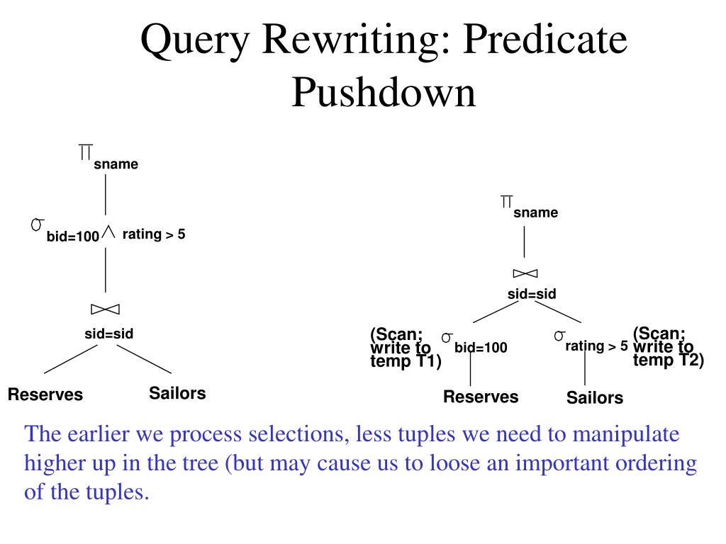
The performance impact of this single heuristic can be enormous.

Predicate Pushdown in Practice

While the concept is simple, the implementation has important nuances, especially concerning different join types. Since you're interested in systems internals, let's look at how a real system like StarRocks applies these rules.

This distinction is a great example of an engineering trade-off. The optimizer applies a powerful general heuristic (push down predicates) but must do so carefully to preserve the exact semantics of the SQL query.

Join Reordering: Finding the Best Path

For queries that join multiple tables, the order in which the joins are performed is another huge factor in performance. The goal is to join tables in an order that keeps the intermediate results as small as possible. This typically means performing the most selective joins (those that produce the fewest rows) first.

Consider a join between tables A, B, and C. A logical plan can execute this as (A ⋈ B) ⋈ C or A ⋈ (B ⋈ C). These are logically equivalent due to the associativity of joins. Furthermore, A ⋈ B is equivalent to B ⋈ A (join commutativity). Together, these properties open up a large search space of possible join orders.

For an N-table join, the number of possible join orders can be very large (related to Catalan numbers). Exhaustively checking every single one is often infeasible. Therefore, optimizers use heuristics and algorithms to explore this space.

From a systems perspective, a common approach is to identify a sequence of INNER JOINs and treat them as a single "multi-join" block to be reordered.

A Better Approach: The Join Graph

In the last lesson, we discussed translating SQL into a "canonical" tree with cross products at the bottom. We then saw how rule-based optimization works hard to transform this tree into something better. This raises a design question: is starting with that canonical tree the best idea in the first place?

Modern optimizers often take a more direct approach. Instead of building an initial tree, they parse the SQL query directly into a join graph, where relations are nodes and join predicates are edges. This representation avoids creating artificial problems (like large cross products) that then need to be fixed.

This shift from a rigid tree to a more flexible graph representation is a powerful design principle. It allows the optimizer to focus directly on the hardest part of the problem—finding the best join order—without being constrained by an arbitrary initial plan structure.

Other Important Logical Transformations

While predicate pushdown and join reordering are the heavy hitters, several other logical transformations are crucial for a complete optimizer.

• Projection Pushdown: Similar to predicate pushdown, this rule pushes projection (π) operators down the tree. This makes tuples "narrower" by discarding unused columns early, which can save significant I/O and memory, especially in a row-oriented system.
• Subquery Decorrelation: Correlated subqueries (where the inner query depends on the outer query) can be very inefficient if executed naively (i.e., re-running the subquery for every outer row). Decorrelation is a set of rewrite rules that transform a correlated subquery into an equivalent JOIN. This allows the subquery to be executed once and enables it to participate in join reordering with the other tables.

SELECT S.sname
FROM Sailors S, Reserves R, Boats B
WHERE S.sid = R.sid AND R.bid = B.bid
  AND B.color = 'red' AND S.age > 30;

Conclusion

In this lesson, you've learned how a query optimizer uses logical transformations to rewrite a query plan. These rule-based heuristics are the first line of defense against inefficient query execution.

Key Takeaways:

• Logical optimization rewrites a query plan using equivalence rules to find a more efficient, but semantically identical, plan.
• Predicate Pushdown is the most important heuristic: filter data as early as possible to reduce the size of intermediate results.
• Join Reordering is critical for multi-table queries. The goal is to find an order that minimizes the size of the data being joined at each step.
• Modern optimizers often bypass the classic "canonical plan" by translating SQL directly into a join graph, which provides a more flexible structure for optimization.
• Other rules like projection pushdown and subquery decorrelation are also essential tools in the optimizer's toolkit.

Preview of the Next Lesson

So far, our rules have been based on heuristics (e.g., "pushing selections is good"). But to choose between two plausible plans (like A ⋈ B vs. B ⋈ A), the optimizer needs more information. It needs to estimate the cost of each alternative. In the next lesson, you will learn how to estimate the cardinality of query results using statistics and selectivity, which is the foundation of cost-based optimization.