Hello! Welcome back to our course on database systems.
In our first lesson, we explored the high-level architecture of a DBMS. We established that its design is heavily influenced by the need to manage the enormous performance gap between fast, volatile main memory and slower, non-volatile disk. This lesson zooms in on that very gap.
Today, we will dig into the "why" behind those architectural choices by comparing the performance characteristics of Hard Disk Drives (HDDs), Solid-State Drives (SSDs), and main memory (DRAM). Understanding these fundamental differences is crucial, as they dictate how we design efficient data structures, indexes, and algorithms for the entire system.
The Storage Hierarchy: A Recap
Let's quickly revisit the storage hierarchy. As we move further from the CPU, storage gets cheaper and larger, but also significantly slower.
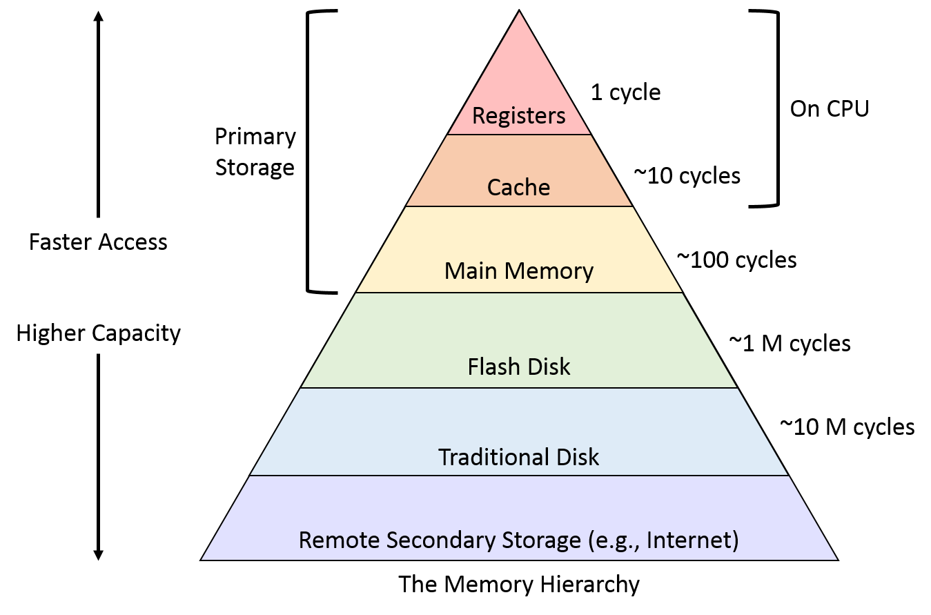
The Great Divide: Latency by the Numbers
The most striking difference between these storage tiers is latency—the time it takes to access a piece of data. The numbers are so vastly different that it can be hard to grasp their scale.
To build your intuition, let's watch a segment from a CMU Database Systems lecture that uses a powerful analogy to make these latencies tangible.
CMU Database Systems - 06 Database Storage (Fall 2017)
This clip from the 'CMU Database Systems' lecture series provides an excellent analogy to help you appreciate the staggering difference in access times between memory and disk.
Please watch from 14:35 to 16:28. The lecturer scales up access times, equating one nanosecond to one second, to illustrate just how slow disk access is in human terms.
As you just saw, waiting for disk is not just "slower"—it's an entirely different category of operation. If a CPU operation took one second, a disk access would take weeks. This is the single most important constraint in a disk-oriented database system.
Let's look at the approximate numbers behind that analogy.
Lecture #02 - In-Memory Databases [CMU Database Systems Spring 2016]
The following clip, from another CMU lecture, provides concrete latency numbers for different storage media. This will give you the quantitative data to back up the analogy.
Watch from 29:20 to 31:12. Pay close attention to the order-of-magnitude jumps between DRAM, SSDs, and HDDs. Note the difference between read and write speeds for SSDs.
Here's a summary of those typical latencies:
| Storage Type | Typical Access Time | Key Characteristics |
|---|---|---|
| DRAM (Memory) | ~60-100 ns | Volatile, byte-addressable, fastest random and sequential access. |
| SSD (Flash) | ~20,000 - 50,000 ns | Non-volatile, block-addressable, reads are faster than writes, fast random I/O. |
| HDD (Disk) | ~10,000,000 ns | Non-volatile, block-addressable, extremely slow random I/O due to mechanical parts. |

Random vs. Sequential Access: The Core Distinction
The table above hints at another critical performance dimension: the pattern of access.
- Sequential Access: Reading data that is stored contiguously, one block after another. Think of reading a book from start to finish.
- Random Access: Reading data from arbitrary, non-contiguous locations. Think of jumping to random pages in a book.
For HDDs, this difference is monumental. An HDD has a mechanical arm that must physically move (a "seek") to the correct track and wait for the platter to spin to the right sector. This physical movement dominates the access time. Therefore, sequential reads are vastly cheaper because the arm can read a long stream of data after only one initial seek.
For SSDs, which have no moving parts, the penalty for random access is much, much lower than for an HDD. While not entirely free (due to internal controller logic), it is orders of magnitude better.
This fundamental difference between HDDs and SSDs has profound implications for how database software is designed.
When Old Optimizations Become New Problems
Your background in algorithms has taught you that an optimization is only as good as the assumptions it's built on. For decades, DBMS developers built systems on one primary assumption: random disk I/O is the ultimate bottleneck, and we must avoid it at all costs.
This led to ingenious algorithms designed to turn random I/O patterns into sequential ones. But what happens when you run this software on modern SSDs, where the initial assumption is no longer as true?
A fascinating paper from the VLDB conference explores these "performance mismatches." You don't need to read the whole paper, but we'll use its findings to see how device characteristics impact real database workloads.
1. The Cost of Sequentiality
A classic HDD-era optimization is to buffer random writes in memory, sort them, and then write them to disk as a single sequential operation.
When Database Meets New Storage Device
Let's examine a key finding from the paper 'When Database Meets New Storage Device'. This section shows how an optimization designed for HDDs can be ineffective or even harmful on SSDs.
Please read Section 3.4, 'Mismatch in I/O Sequentiality'. Focus on the text and the two charts in Figure 6. The left chart shows the performance impact of this optimization on an HDD vs. an SSD. The right chart shows the CPU cost, which helps explain the 'why'.
As the paper shows, the CPU cost of converting random I/Os to sequential ones can outweigh the small benefit gained on an SSD, where random I/O is already fast. The optimization, which is a clear win on an HDD, becomes a wash or even a slight loss on an SSD.
2. The Penalty of Small Writes
Database workloads, especially transactional ones (OLTP), often involve many small, frequent updates that must be durably written to disk (e.g., committing a transaction).
When Database Meets New Storage Device
Now, let's look at another mismatch from the same paper. This one concerns I/O size.
Please read the 'Symptom' paragraph in Section 3.2, 'Mismatch in I/O Size', and look at Figure 3. This figure dramatically illustrates how performance on NVMe SSDs collapses with frequent, small writes compared to SATA SSDs and HDDs.
This happens because SSDs operate internally on larger units (cache lines and erase blocks). Frequent, small, forced writes (fsync) can disrupt the drive's internal logic, leading to inefficiencies and significant performance degradation that is far more severe than on an HDD.
Test your understanding!
Imagine you are designing a system to store time-series data from IoT sensors. The primary workload consists of millions of tiny, independent writes per minute as new data arrives. Based on what you've just learned, which storage characteristic would be your biggest concern if you were forced to use an older, HDD-optimized database system on a modern NVMe SSD?
Show answer
The biggest concern would be the mismatch in I/O size. The database system, designed for HDDs, would likely try to force each small write to disk to ensure durability. As shown in the VLDB paper (Figure 3), this pattern of frequent, small, forced writes is catastrophic for NVMe SSD performance. The system would be better served by an architecture designed to batch these small writes into larger chunks before flushing, a key feature of modern systems like Log-Structured Merge-Trees (LSM-Trees), which we'll cover later in the course.
The Main Memory Fallacy
Given how slow disk is, what if we just use a machine with enough RAM to hold the entire database? You might assume that a disk-oriented DBMS would simply fly in this scenario. However, the performance characteristics of the assumed storage medium are baked deep into the system's architecture.
Lecture #02 - In-Memory Databases [CMU Database Systems Spring 2016]
This final video clip shows where the CPU cycles are actually spent in a disk-oriented DBMS, even when all the data fits in memory. The results are surprising and highlight the overhead of an architecture built for disk.
Please watch from 17:33 to 19:50. The pie chart is the key takeaway. It shows how little time is spent on 'useful work' versus managing components like the buffer pool and locks, which exist primarily to mitigate disk latency.
Even with zero disk I/O, a huge fraction of CPU time is spent on the machinery built to avoid disk I/O—managing the buffer pool, checking if pages are in memory, and handling locks. This demonstrates that performance isn't just about the raw speed of the hardware, but about designing algorithms that align with that hardware's characteristics. An in-memory database requires a fundamentally different architecture to be truly efficient.
Conclusion
In this lesson, we quantified the massive performance differences between main memory, SSDs, and HDDs, and explored how these characteristics shape database system design.
Key Takeaways:
- Orders of Magnitude: The latency gap between memory, SSDs, and HDDs is not incremental; it spans many orders of magnitude.
- Random vs. Sequential: This is the defining performance axis for disk. HDDs are crippled by random access due to mechanical delays, while SSDs are far more efficient.
- Workload Matters: The performance of a storage device is not a single number. It depends on the access pattern (random vs. sequential), I/O size, and parallelism of the workload.
- Architecture is Tied to Hardware: Database systems are highly optimized for a specific storage medium. An architecture designed for HDDs carries significant overhead and may even employ anti-patterns when run on modern SSDs.
Preview of the Next Lesson:
Now that we understand the constraints and characteristics of the underlying disk, our next step is to learn how a DBMS actually organizes data on it. In the next lesson, we will design a page layout for storing fixed-length and variable-length records (slotted pages). This is the first fundamental data structure we will build in the storage layer.