B+ Tree Indexing vs. Full Table Scan: A Cost Analysis

Hello! Welcome to the first lesson of our module on Query Execution.

In the previous module, we took a deep dive into the internal structure of indexing data structures, focusing on B+ Trees and hash indexes. You learned how they are built, maintained, and the trade-offs between them.

Now, we move up one layer in the database architecture to see how the system uses these indexes to execute queries. We'll start with the most fundamental operation: selection, which corresponds to the WHERE clause in an SQL query.

Today's lesson will focus on implementing and analyzing an index-based selection operator. By the end of this 60-minute session, you will be able to explain how to use a B+ tree to find records matching a predicate and analyze its I/O cost compared to a simple full table scan. This is the first step in understanding how a declarative SQL query is translated into an efficient, executable plan.

1. The Selection Operator and the Baseline: Full Table Scan

A selection operator is a relational algebra operator that filters a set of records, returning only those that satisfy a given condition (a predicate). In SQL, this is the job of the WHERE clause.

The simplest, most straightforward way to implement selection is with a full table scan (or sequential scan). The algorithm is exactly what it sounds like:

Start at the first page of the table file.
For each record on the page, check if it satisfies the predicate.
If it does, add it to the result set.
Move to the next page and repeat until all pages have been scanned.

This approach is simple to implement and is guaranteed to find all matching records. But what is its cost? To analyze this, we'll use a simple I/O cost model.

I/O Cost Model, Tree Indexes

These lecture slides from the University of Massachusetts Boston introduce a simple and effective I/O cost model that we'll use throughout this module. It helps us reason about the performance of different algorithms.

Please read the slides titled 'Cost Model and Performance Analysis' and 'Cost Model: Heap Files (unsorted)'. Focus on understanding the key parameters, especially: B: The number of data pages in the file. D: The average time to read or write a single disk page. Pay attention to the calculated I/O cost for a 'Scan' operation on a heap file.

As the slides explain, the cost of a full table scan is simply B * D. If your table occupies B pages on disk, you must perform B disk I/Os to read the entire thing. This is our baseline. Any other approach must be better than B * D to be considered an optimization.

2. The Optimized Path: Index-Based Selection

A full table scan is inefficient if the predicate is highly selective—that is, if only a tiny fraction of records match. For example, if you're looking for a single user by their unique ID in a table with a billion users, reading the entire table is enormously wasteful.

This is where our B+ Tree index comes in. Instead of scanning the table, we can use the index to directly locate the records we need.

The general algorithm for an index-based selection is a two-step process:

Use the B+ tree to find the (key, RID) pairs that satisfy the predicate. A RID (Record ID) is a pointer (e.g., page ID + slot number) to the location of the actual tuple.
For each RID found, fetch the corresponding data page from the table file and retrieve the tuple.

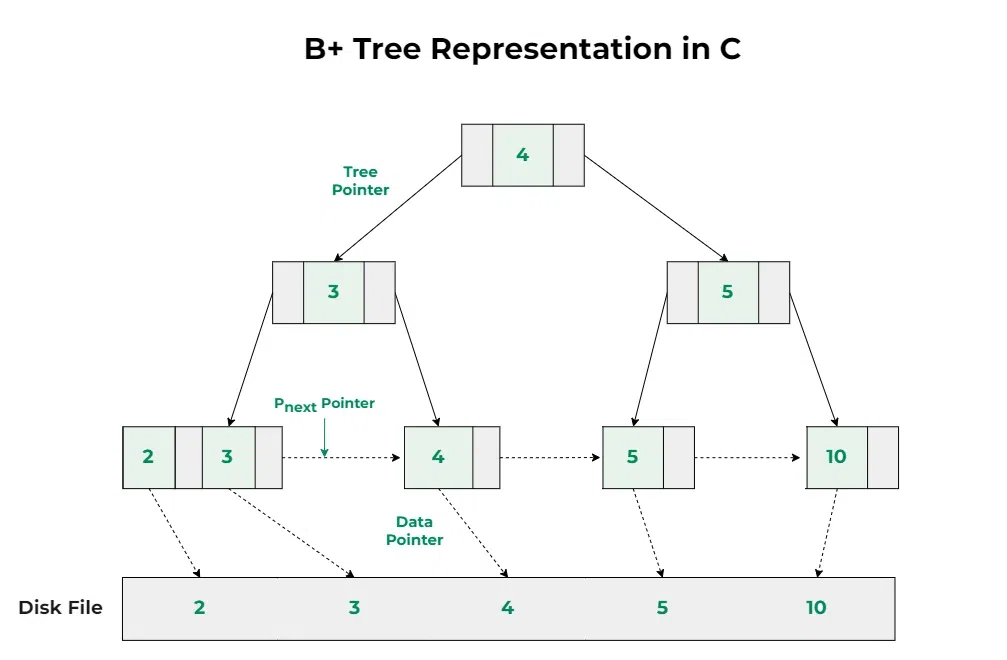
B+ Tree Conceptual Representation — This diagram shows the core idea. The B+ Tree (top) allows us to find keys efficiently. The leaf nodes contain 'Data Pointers' (our RIDs) that point to the actual records in the 'Disk File' (bottom).

The specific mechanics of Step 1 depend on the type of predicate.

Equality Predicates (`WHERE column = value`)

For a point query, we perform a standard search on the B+ tree:

Start at the root page.
Follow the child pointers down the tree based on key comparisons.
Arrive at the correct leaf page that should contain the key.
Search the leaf page for the key and retrieve its associated RID.

Range Predicates (`WHERE column > value` or `BETWEEN val1 AND val2`)

For a range query, we leverage the sorted, linked-list structure of the leaf pages:

Perform a search on the B+ tree to find the leaf page containing the start of the range (val1).
Retrieve all matching RIDs from that page.
Follow the sibling pointer to the next leaf page.
Continue scanning across leaf pages, collecting RIDs, until you pass the end of the range (val2).

Test your understanding!

Imagine you're implementing the selection operator in C++. How would the B+ tree data structure you've designed support these two types of selections? What methods would your BPlusTree class need to expose?

Show answer

Your B+ Tree implementation would need to provide two key pieces of functionality, which map directly to the CMU project specification (LINK):

For equality predicates: A GetValue(key, &rids) or similar method that performs a point search and returns the list of RIDs for a given key. This corresponds to Task #2 in the project description.
For range predicates: An Iterator class. You would initialize the iterator to the start of the range (begin(start_key)). You could then use a ++ operator to move through the sorted leaf pages, accessing each (key, RID) pair until you reach the end of the range. This corresponds to Task #3, the Index Iterator.

3. Cost Analysis: Index Scan vs. Full Table Scan

Now for the crucial question: when is an index scan actually faster? The answer depends heavily on the cost of the two steps (finding RIDs and fetching data) and whether the index is clustered or unclustered.

I/O Cost of an Index Scan

Let h be the height of the B+ Tree.

Tree Traversal: The cost to find the first leaf page is h * D. B+ trees are very shallow; a height of 3 or 4 can index billions of records. So, this cost is typically just 3-4 I/Os.
Data Fetching: This is where the cost varies dramatically. Let k be the number of tuples that match the predicate.

Scenario 1: Unclustered Index (The Common Case)
In an unclustered index, the physical order of data rows on disk has no relationship to the index order. The RIDs in the index leaves can point to random pages all over the table file.

Cost: In the worst case, each of the k matching tuples is on a different data page. This results in k random disk I/Os.
Total Cost (Unclustered): (h * D) + (k * D)

The problem of fetching many random pages is often called pointer chasing and can be very expensive.

Scenario 2: Clustered Index
In a clustered index, the data rows themselves are sorted and stored in the same order as the index keys (often, the leaf pages of the index are the data pages).

Cost: Because the data is sorted, all k matching tuples will be located physically next to each other on a small number of contiguous pages. Let's say these tuples fit onto P_data pages.
Total Cost (Clustered): (h * D) + (P_data * D)

Since P_data is typically much, much smaller than k, a clustered index is significantly more efficient for range scans.

This video from CMU explains the performance implications and a clever optimization.

#08 - Tree Indexes: B+Trees (CMU Intro to Database Systems)

Professor Pavlo discusses the crucial performance difference between clustered and unclustered indexes for scans.

Watch the segment from 00:55:07 to 00:58:44. Focus on why an unclustered index scan can lead to costly random I/O, and note the optimization he describes: collecting all the RIDs first, sorting them by page ID, and then fetching the pages.

The Optimizer's Choice

So, when should the system use an index scan versus a full table scan? The query optimizer makes this decision by estimating the cost of both plans. For an unclustered index, the choice is between:

Full Table Scan Cost: B * D
Index Scan Cost: (h + k) * D

The decision hinges on the selectivity of the predicate:

High Selectivity (small k): If you're fetching just a few rows (k is small), h + k will be much less than B. The index scan is the clear winner.
Low Selectivity (large k): If your query matches a large percentage of the table (e.g., WHERE age > 20 in a university database), k can be very large. It might be cheaper to just scan all B pages sequentially than to do k random I/Os. In this case, the optimizer will wisely choose a full table scan, even if an index is available.

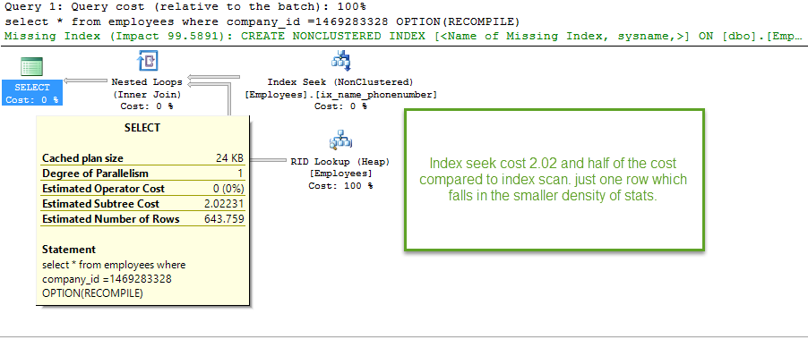
This EXPLAIN plan from a real query demonstrates the optimizer's choice in action.

08 - B+Tree Indexes (CMU Intro to Database Systems / Fall 2022)

In this demo from a previous CMU lecture, watch how PostgreSQL's optimizer chooses between an index scan and a sequential scan based on the predicate's selectivity.

Watch from 01:15:30 to 01:19:42. Notice that WHERE email LIKE 'foo%' (low selectivity, matches many common emails) results in a Sequential Scan. But WHERE email LIKE 'zzz%' (high selectivity, matches few emails at the end of the alphabetical range) results in an Index Scan. This is the cost-based decision in practice.

The execution plan below shows what an index-based selection looks like.

SQL Server Query Execution Plan with Index Seek Cost Analysis — This query plan from SQL Server shows an 'Index Seek' operation, which is the B+ tree traversal. This feeds into a 'RID Lookup', which is the second step of fetching the actual data from the table heap. The optimizer has estimated the cost and decided this two-step process is cheaper than a full scan.

Summary

Let's tie everything together. You now understand the two primary ways a database system can execute a selection operation.

Key Takeaways:

Full Table Scan: The baseline approach. It reads every page of the table. Its I/O cost is B * D, where B is the total number of pages in the table.
Index Scan: A two-step process. First, traverse the B+ tree to find the Record IDs (RIDs) of matching tuples. Second, use the RIDs to fetch the tuples from the data pages.
Cost is King: The query optimizer chooses between these plans by estimating their I/O cost. The key factors are the predicate's selectivity (how many rows will match) and whether the index is clustered or unclustered.
The Unclustered Index Trap: For a low-selectivity query, using an unclustered index can be slower than a full table scan because the cost of numerous random I/Os to fetch data (k * D) can exceed the cost of reading the whole table sequentially (B * D).

Preview of the Next Lesson

We've covered how to filter data using the WHERE clause. What about ORDER BY? In the next lesson, we will tackle External Merge Sort, a fundamental algorithm for sorting datasets that are too large to fit into main memory. This algorithm is not only crucial for handling ORDER BY clauses but is also a key building block for more complex operators, like sort-merge join.

Recommended resources