Real-time P&L and Greeks Monitoring Function

1. Recap: The Data We Need

Let's look back at the manage_position method we developed. It needs the following real-time data to make decisions:

• Cost to Close: To evaluate profit targets and stop-losses. This is derived from the current bid/ask prices of the legs.
• Net Delta: To trigger adjustments when directional risk gets too high.
• Days to Expiration (DTE): To trigger time-based adjustments.
• Profit & Loss (P&L): While we used cost_to_close to calculate P&L, Interactive Brokers also provides a direct P&L stream.

Our goal is to create a monitoring function that fetches these values from the broker API and makes them available to our strategy. We will focus on two primary streams of information: P&L and the option Greeks.

2. Monitoring Position P&L with ib_insync

Interactive Brokers provides a direct way to subscribe to P&L updates for your entire account or for a single position. For our framework, where a strategy instance manages a specific spread, monitoring a single position's P&L is the most direct and efficient approach.

The ib_insync library offers the ib.reqPnLSingle() method for this purpose. It establishes a subscription for a specific position (identified by an account, model code, and contract ID) and provides continuous updates.

Let's consult the ib_async documentation for a related example.

The key insight from the documentation is the event-driven approach. You don't repeatedly ask for the P&L; you subscribe once and then listen for updates.

Here’s how we can adapt that pattern to create a function that subscribes to P&L updates for our spread position. Note that to monitor a combo/spread position, we would typically monitor the P&L of each leg individually.

# In a new file, e.g., framework/monitoring.py
from ib_insync import IB, PnLSingle

def subscribe_to_pnl_updates(ib: IB, account: str, position: dict, pnl_data: dict):
    """
    Subscribes to P&L updates for each leg of a spread position.
    
    Args:
        ib: The connected IB instance.
        account: The account number.
        position: The position object containing contract details.
        pnl_data: A dictionary to store the P&L objects.
    """
    
    def on_pnl_update(pnl: PnLSingle):
        """Callback to handle incoming P&L updates."""
        # We can identify the leg by its conId
        pnl_data[pnl.conId] = pnl
        print(f"P&L Update for conId {pnl.conId}: Unrealized PnL: {pnl.unrealizedPnL:.2f}")

    # Subscribe for the short leg
    short_leg_contract = position['short_leg']['contract']
    ib.reqPnLSingle(account, '', short_leg_contract.conId)
    
    # Subscribe for the long leg
    long_leg_contract = position['long_leg']['contract']
    ib.reqPnLSingle(account, '', long_leg_contract.conId)

    # Attach the event handler
    ib.pnlSingleEvent += on_pnl_update

    print("Subscribed to P&L updates for position legs.")

In this setup, pnl_data is a shared dictionary that gets populated with PnLSingle objects as the broker sends updates. Our main monitoring loop can then read from this dictionary to get the latest P&L for each leg and sum them for the total position P&L.

3. Monitoring Position Greeks

Unlike P&L, there isn't a single subscription for a spread's aggregated Greeks. Instead, we get the Greeks for each individual option leg as part of their real-time market data stream. We then calculate the spread's net Greeks ourselves.

Your background in options fundamentals will be useful here. The net Greek of a spread is the sum of the Greeks of its components, being mindful of the sign (long vs. short positions). For our credit spreads:

• Net Delta = Delta of Short Leg + Delta of Long Leg
• Net Gamma = Gamma of Short Leg + Gamma of Long Leg
• Net Theta = Theta of Short Leg + Theta of Long Leg
• Net Vega = Vega of Short Leg + Vega of Long Leg

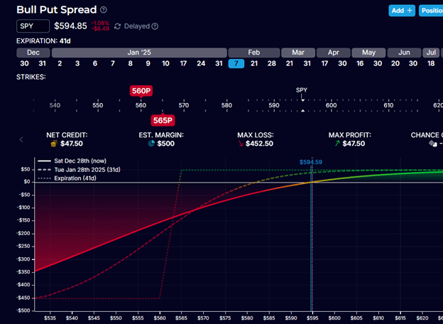
Since we are short one option and long another, their Greeks will partially offset. For a bull put spread (short a put, long a lower-strike put), the calculation is effectively (delta_of_short_put) - (delta_of_long_put). Since put deltas are negative, this results in a net positive delta, which is what we expect.

To see how ib_insync provides this data, let's watch a short video.

As the video demonstrates, the process is:

1. Request market data for an option contract using ib.reqMktData().
2. The returned Ticker object will be continuously updated by the API.
3. The Greeks are available in the ticker.modelGreeks attribute.

We can now write a function to subscribe to this data for both legs of our spread.

# In framework/monitoring.py
from ib_insync import IB, Ticker

def subscribe_to_market_data(ib: IB, position: dict, ticker_data: dict):
    """
    Subscribes to market data for each leg of a spread position.

    Args:
        ib: The connected IB instance.
        position: The position object containing contract details.
        ticker_data: A dictionary to store the Ticker objects.
    """
    
    def on_ticker_update(ticker: Ticker):
        """Callback to handle incoming market data updates."""
        # Ticker updates don't always contain modelGreeks, so check for it
        if ticker.modelGreeks:
            # We can identify the leg by its conId
            ticker_data[ticker.contract.conId] = ticker
            # Optional: print a confirmation
            # print(f"Greeks update for {ticker.contract.conId}: Delta {ticker.modelGreeks.delta}")

    # Request market data for both legs
    short_leg_contract = position['short_leg']['contract']
    long_leg_contract = position['long_leg']['contract']
    
    ib.reqMktData(short_leg_contract, '', False, False)
    ib.reqMktData(long_leg_contract, '', False, False)

    # Attach the event handler to the generic pending tickers event
    ib.pendingTickersEvent += on_ticker_update

    print("Subscribed to market data for position legs.")

4. The Continuous Monitoring Function

Now we can combine everything into the main monitoring function. This function's job is to read the latest data from our subscriptions and update a central position_state object. The manage_position method will then read from this object. This approach decouples data collection from decision logic.

# In framework/monitoring.py
import asyncio
from ib_insync import util

# (include the subscription functions from above)

async def continuously_monitor_position(ib: IB, account: str, position: dict, position_state: dict):
    """
    Continuously monitors P&L and Greeks for an open position.
    
    Args:
        ib: The connected IB instance.
        account: The account number.
        position: The static position data (contracts, entry price).
        position_state: A dictionary to be continuously updated with live data.
    """
    # Dictionaries to hold the live data objects from callbacks
    pnl_data = {}
    ticker_data = {}

    # Set up the subscriptions
    subscribe_to_pnl_updates(ib, account, position, pnl_data)
    subscribe_to_market_data(ib, position, ticker_data)
    
    # Allow some time for initial data to arrive
    await asyncio.sleep(5)

    while True:
        # Check if we have data for both legs
        short_conId = position['short_leg']['contract'].conId
        long_conId = position['long_leg']['contract'].conId

        if short_conId in pnl_data and long_conId in pnl_data and \
           short_conId in ticker_data and long_conId in ticker_data:
            
            short_pnl = pnl_data[short_conId]
            long_pnl = pnl_data[long_conId]
            
            short_ticker = ticker_data[short_conId]
            long_ticker = ticker_data[long_conId]

            # --- 1. Update P&L ---
            unrealized_pnl = short_pnl.unrealizedPnL + long_pnl.unrealizedPnL
            position_state['unrealized_pnl'] = unrealized_pnl
            
            # --- 2. Update Greeks ---
            if short_ticker.modelGreeks and long_ticker.modelGreeks:
                # Note: For a short position, you are short the greeks.
                # A bull put is SHORT a put and LONG a lower strike put.
                # Net Delta = (Delta of the put you are short) - (Delta of the put you are long)
                # This correctly reflects your net directional exposure.
                net_delta = short_ticker.modelGreeks.delta - long_ticker.modelGreeks.delta
                net_gamma = short_ticker.modelGreeks.gamma - long_ticker.modelGreeks.gamma
                net_theta = short_ticker.modelGreeks.theta - long_ticker.modelGreeks.theta
                net_vega = short_ticker.modelGreeks.vega - long_ticker.modelGreeks.vega
                
                position_state['greeks'] = {
                    'delta': net_delta,
                    'gamma': net_gamma,
                    'theta': net_theta,
                    'vega': net_vega,
                }
            
            # --- 3. Update Current Price ---
            # Cost to close = (price to buy back short leg) - (price to sell long leg)
            cost_to_close = short_ticker.ask - long_ticker.bid
            position_state['cost_to_close'] = cost_to_close
            
            # Optional: Log the updated state
            # print(f"State Update: P&L={unrealized_pnl:.2f}, Delta={net_delta:.3f}")

        await asyncio.sleep(1) # Check for updates every second

This asynchronous function runs in the background. It sets up the data streams and then enters a loop, continuously calculating and updating the position_state object. Your main trading loop can then pass this position_state object to the manage_position method, which now has all the live data it needs.

Conclusion

Congratulations! You have now built the complete feedback loop for managing an open position. We've gone from defining high-level rules like "take profit at 50%" to implementing the low-level functions that provide the real-time data needed to enforce those rules.

Key Takeaways:

• Live position monitoring involves subscribing to data streams rather than repeatedly polling for data.
• We use ib.reqPnLSingle to get real-time P&L updates for each leg of our spread.
• We use ib.reqMktData to get market data for each leg, which includes the Greeks via the ticker.modelGreeks attribute.
• Net spread Greeks are calculated by combining the Greeks of the individual legs, accounting for short and long positions.
• A dedicated, asynchronous monitoring function is a clean way to manage data streams and update a shared state object for the strategy logic to consume.

Preview of the Next Lesson:
With the entry, management, and exit logic for a credit spread now fully defined, our framework can handle a trade from start to finish. The final question is: what triggers the trade in the first place? In our next module, we will shift our focus to signal generation. The first lesson will be to design an abstract SignalGenerator class to create a pluggable interface for different entry signals, allowing us to experiment with various indicators and market conditions to initiate our trades.