Implied Volatility Calculation

What is Implied Volatility?

You're already familiar with the Black-Scholes model, which calculates an option's theoretical price based on several inputs: the underlying price, strike price, time to expiration, risk-free rate, and volatility.

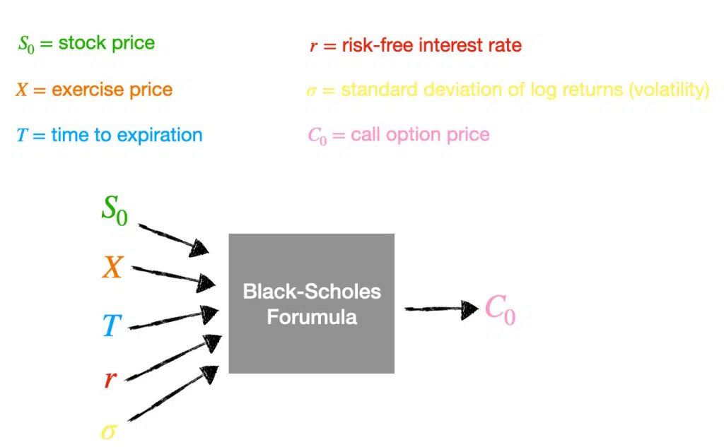
Of all these inputs, volatility is the only one not directly observable. Implied volatility (IV) is the value of volatility that, when plugged into the Black-Scholes formula, yields the option's current market price. In essence, it's the market's consensus on the underlying asset's future volatility, "implied" by the option's price.

The challenge is that the Black-Scholes formula cannot be algebraically rearranged to solve for volatility. We need a numerical method to find it.

The Newton-Raphson Method for Implied Volatility

Given your background in mathematics, you'll appreciate the elegance of the Newton-Raphson method, a highly efficient root-finding algorithm. This is the standard approach for calculating implied volatility.

The core idea is to find the root of the following function, f(σ):

$f(\sigma )={\text{Price}}_{BS}(\sigma )-{\text{Price}}_{Market}$

We are looking for the value of $\sigma$ that makes this function equal to zero. The Newton-Raphson method does this iteratively:

1. Start with an initial guess for volatility, ${\sigma }_{old}$.
2. Calculate a new, better guess, ${\sigma }_{new}$, using the formula:
   ${\sigma }_{new}={\sigma }_{old}-\frac{f({\sigma }_{old})}{f^{\prime }({\sigma }_{old})}$
3. Repeat until the difference between ${\sigma }_{new}$ and ${\sigma }_{old}$ is smaller than a specified tolerance.

For our problem:

• $f({\sigma }_{old})$ is the difference between the Black-Scholes price calculated with our guess and the actual market price.
• $f^{\prime }({\sigma }_{old})$ is the derivative of the Black-Scholes price with respect to volatility. This is one of the Greeks you're familiar with: Vega.

The following video from the QuantPy channel provides an excellent, concise walkthrough of this exact process and implements it in Python using the py_vollib library, which we are already using in our project.

Implementing the Function

As you saw in the video, the implementation involves a loop that iteratively refines the volatility estimate. Let's integrate this logic into our OptionsAnalytics class.

Here is the implementation of the calculate_implied_volatility static method. Note that it uses our existing calculate_greeks function's dependencies (black_scholes and vega from py_vollib).

# In framework/analytics.py

# ... (existing imports)

class OptionsAnalytics:
    """
    A utility class to encapsulate options pricing and Greek calculations
    using the py_vollib library.
    """
    
    # ... (existing calculate_greeks and calculate_aggregated_greeks methods) ...

    @staticmethod
    def calculate_implied_volatility(
        market_price: float, 
        flag: str, 
        S: float, 
        K: float, 
        t: float, 
        r: float,
        tolerance: float = 0.0001,
        max_iterations: int = 100
    ) -> float:
        """
        Calculates the implied volatility of an option using the Newton-Raphson method.

        Args:
            market_price (float): The market price of the option.
            flag (str): 'c' for call, 'p' for put.
            S (float): Current underlying asset price.
            K (float): Strike price.
            t (float): Time to expiration in years.
            r (float): Risk-free interest rate.
            tolerance (float): The desired precision of the result.
            max_iterations (int): The maximum number of iterations.

        Returns:
            float: The implied volatility, or 0.0 if not found.
        """
        # Initial guess for volatility
        sigma = 0.5  

        for i in range(max_iterations):
            # Calculate option price and vega with the current sigma guess
            price_at_sigma = black_scholes(flag, S, K, t, r, sigma)
            
            # As noted in the video, py_vollib's vega is for a 1% change, 
            # so we multiply by 100 to get the raw derivative.
            vega_at_sigma = vega(flag, S, K, t, r, sigma) * 100

            # Difference between model price and market price
            price_diff = price_at_sigma - market_price

            # Check if we are close enough
            if abs(price_diff) < tolerance:
                return sigma

            # Avoid division by zero
            if vega_at_sigma == 0:
                # Cannot converge if vega is zero, return last guess or handle as error
                return sigma  

            # Newton-Raphson iteration step
            sigma = sigma - price_diff / vega_at_sigma
        
        # If max iterations reached without converging, return last guess or indicate failure
        return sigma

Example Usage

Let's test our new function. We'll first calculate a theoretical price with a known volatility, then use our function to see if we can recover that original volatility.

# --- Example Usage ---

# Define option parameters
S = 100.0
K = 105.0
t = 30 / 365.0
r = 0.05
flag = 'c'
known_sigma = 0.35 # Our "true" volatility

# 1. Calculate the market price using a known sigma
market_price = black_scholes(flag, S, K, t, r, known_sigma)
print(f"Theoretical market price for sigma={known_sigma}: {market_price:.4f}")

# 2. Now, calculate the implied volatility from that market price
iv = OptionsAnalytics.calculate_implied_volatility(market_price, flag, S, K, t, r)
print(f"Calculated Implied Volatility: {iv:.4f}")

# Expected Output:
# Theoretical market price for sigma=0.35: 0.8033
# Calculated Implied Volatility: 0.3500 

The function successfully calculates that an option with a market price of $0.8033 has an implied volatility of 35%, matching our original input.

The Production-Ready Shortcut: py_vollib's Built-in Function

While implementing the Newton-Raphson method is an excellent exercise for understanding the mechanics, for our actual trading framework, it's wiser to use the highly optimized and robust implementation provided directly by py_vollib. This function handles edge cases and uses a faster, more stable algorithm (LetsBeRational).

Learning about this built-in function will save you development time and prevent potential numerical issues.

As you can see from the documentation, the library provides a simple, direct function call. For our framework, we can create a wrapper around this function inside our OptionsAnalytics class for consistency. This gives us the best of both worlds: a clean internal API and a professionally implemented backend.

Conclusion

Today we have closed a critical loop in our analytics engine. We started with the knowledge that implied volatility is a key input for our Greek calculations, and we have now built the tool to derive it directly from market prices.

Key Takeaways:

• Implied volatility is the market's expectation of future price movement, calculated by "inverting" the Black-Scholes model.
• Since there is no direct algebraic solution, numerical methods like Newton-Raphson are required. This method iteratively refines a guess for volatility until the model price matches the market price.
• The core of the Newton-Raphson iteration relies on Vega, the option's sensitivity to volatility.
• While it's valuable to understand how to implement the algorithm, production systems should rely on optimized library functions like py_vollib.black_scholes.implied_volatility.implied_volatility.

Preview of the Next Lesson:
With our dynamic analytics now complete (Greeks and IV from market prices), we can turn our attention to the static characteristics of our spreads. In the next lesson, we will build functions to compute max profit, max loss, and breakeven points for a given credit spread. These metrics are essential for defining risk limits and profit targets in our strategy logic.