RMSNorm: Simplifying LayerNorm

Introduction

In our last module, we established the foundational architecture of the Transformer and the high-level paradigm of pre-training and fine-tuning. We saw how a powerful, general-purpose base model is created and then aligned to become a helpful assistant model.

Now, we're going to zoom in and dissect the specific architectural choices that make modern Large Language Models (LLMs) like Qwen 2.5, Llama 3, and DeepSeek-V3 so efficient and powerful. The course syllabus refers to these as the "LLaMA-fication of the Transformer block."

Our first learning outcome is to explain RMSNorm and how it simplifies LayerNorm by removing the mean-centering operation. You'll discover how a seemingly small change in a normalization layer can lead to significant gains in computational efficiency, a crucial factor when training models with billions of parameters.

As a brief recap, in the previous module, we learned that Layer Normalization (LayerNorm) is a key component used after the self-attention and feed-forward sub-layers. Its purpose is to stabilize training by standardizing the activations, which involves two main steps:

1. Centering: Subtracting the mean of the activations.
2. Scaling: Dividing by the standard deviation.

Today, we'll challenge the necessity of the first step.

1. The Problem with LayerNorm: Is Centering Redundant?

While LayerNorm is effective, it introduces a computational bottleneck. To normalize any single activation, the model must first compute the mean and standard deviation across all activations in that layer. The calculation of the mean, in particular, creates a dependency that can slow things down. This led researchers to ask a critical question: is the centering step (subtracting the mean) truly necessary?

To explore this, let's read a short article that deconstructs LayerNorm and sets up the hypothesis behind its more efficient successor.

As the article highlights, the key insight is that the network can effectively "undo" the centering operation using its learnable parameters. If the activations are already reasonably centered—a common situation in deep networks with residual connections—then explicitly calculating and subtracting the mean might be wasted effort.

This is the core idea behind Root Mean Square Normalization (RMSNorm).

2. RMSNorm: Scaling without the Center

RMSNorm simplifies LayerNorm by removing the mean-centering operation entirely. It focuses only on re-scaling the activations.

Instead of measuring the spread of data around a calculated mean (standard deviation), RMSNorm measures the magnitude of the data around zero. It does this using the Root Mean Square (RMS) statistic.

The flowchart below provides a great visual summary of this simplification.

Let's look at the formulas side-by-side to make this concrete.

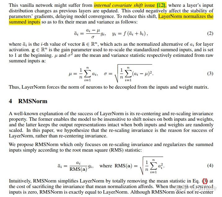
Now, let's dive into the specifics of the RMSNorm formulation.

To summarize, RMSNorm makes a simple but powerful change:

• It removes the mean calculation ($\mu$) and the subsequent centering step ($x-\mu$).
• It removes the learnable shift parameter ($\beta$), as there is no centering to undo.
• It normalizes by the Root Mean Square (RMS) of the input vector, which measures the vector's overall magnitude.

This leaves a purely scaling operation:

where $\gamma$ is a learnable scaling parameter.

3. The Mathematical Connection

You might be wondering how RMS is related to standard deviation ($\sigma$) and how removing the mean ($\mu$) is mathematically justified. Given your preference for balanced theory and application, you'll find the derivation quite elegant.

The relationship between RMS, standard deviation, and the mean can be expressed with an equation that resembles the Pythagorean theorem.

The final formula is remarkably simple:

This tells us everything we need to know:

• If the mean $\mu$ is zero, then $\text{RMS}(x)=\sigma$. In this case, RMSNorm is identical to LayerNorm (without the $\beta$ shift).
• If the mean $\mu$ is small relative to the standard deviation $\sigma$, then $\text{RMS}(x)\approx \sigma$. The two normalizations behave almost identically.

This is precisely why RMSNorm works so well in practice. In large Transformer models, techniques like residual connections help keep the activations naturally centered around zero, making the explicit centering step of LayerNorm largely redundant.

4. The Result: Efficiency and Performance

By removing the mean calculation, RMSNorm is computationally faster and uses fewer parameters than LayerNorm. Let's watch a short video segment that explains the original authors' hypothesis and the practical benefits.

The key benefit is a reduction in computation and memory operations. While a single normalization step is tiny, these steps are performed for every token at every layer. Across billions of training steps or millions of inference requests, these small savings compound into significant improvements in speed and cost, which is why RMSNorm has become the standard in nearly all modern open-source LLMs.

Conclusion

In this lesson, we've dissected RMSNorm, the first of our "modern" Transformer components. You've seen how a principled simplification of a standard architectural piece leads to greater efficiency without sacrificing performance.

Key Takeaways:

• LayerNorm performs two steps: centering (subtracting the mean) and scaling (dividing by standard deviation).
• RMSNorm simplifies this by removing the mean-centering step, hypothesizing that only scaling is necessary for stabilizing deep networks.
• It achieves this by normalizing with the Root Mean Square (RMS) of the input, which measures magnitude around zero.
• The mathematical relationship ${\text{RMS}}^2={\sigma }^2+{\mu }^2$ shows that RMSNorm is equivalent to LayerNorm when the mean $\mu$ is zero.
• This simplification makes RMSNorm computationally faster and more parameter-efficient, leading to its widespread adoption in models like Qwen 2.5 and Llama 3.

Preview of the Next Lesson:
We will continue our exploration of the modern Transformer block by examining the SwiGLU activation function. You'll learn how this gated linear unit enhances the capacity of the Feed-Forward Network (FFN) sub-layer, another key ingredient for building high-performing LLMs.