Tokenizing BEV Features with VQ-VAE

Part 1: From Multi-View Sensors to a Unified BEV Map

An autonomous vehicle is equipped with a suite of sensors—typically multiple cameras, LiDAR, and radar—each providing data from a different perspective and in a different format. A key challenge in 3D perception is fusing this information into a single, coherent representation that the planning system can use.

The most common solution is the Bird's Eye View (BEV) representation. BEV is a top-down 2D grid that represents the scene around the vehicle, much like a satellite map. This unified space is powerful because it resolves the different sensor orientations and makes spatial relationships explicit. Objects that are far away in a camera's perspective view are correctly placed in the BEV grid based on their real-world coordinates.

Creating the BEV Feature Map

The process of converting multi-view camera images into a single BEV feature map is a critical preliminary step before tokenization. This transformation is often called a "lift-splat" or "view-transformation" process. The video below gives an excellent overview of the challenges in 3D perception and the motivation for using BEV, then dives into the technical details of this transformation.

As the video details, the process can be summarized in three steps:

1. Depth Prediction: For each pixel in the 2D camera images, the model predicts a probability distribution over a set of possible depths. This is essential because a 2D image lacks explicit 3D information.
2. "Lift" to 3D Point Cloud: Using the camera's known calibration parameters and the predicted depth distribution, each 2D pixel is "lifted" into a set of 3D points, creating a pseudo-point cloud. The feature for each 3D point is a combination of the original pixel's feature vector and its predicted depth probability.
3. "Splat" onto BEV Grid: These millions of 3D points are then projected onto the top-down 2D BEV grid. All points that fall within the same grid cell are aggregated (e.g., via summation) to produce a single feature vector for that cell.

The final result is a BEV feature map: a 2D grid where each cell contains a rich, continuous feature vector summarizing the semantics of that specific location in the real world. This feature map is the continuous representation we now need to tokenize.

Part 2: Tokenizing the BEV Map with VQ-VAE

Now that we have our BEV feature map, we can see how the VQ-VAE architecture fits into the pipeline. The BEV feature map is an image-like grid of continuous vectors—the perfect input for the VQ-VAE encoder.

Let's briefly recap the VQ-VAE architecture from our last lesson.

The process of tokenizing a BEV map follows these steps precisely:

1. Input: The BEV feature map (e.g., a 200x200 grid of D-dimensional vectors) is fed into the VQ-VAE.
2. Encoder (BEV Patch Embedding): The VQ-VAE's encoder processes the BEV map. Often, it will first divide the map into a grid of smaller patches (e.g., breaking a 200x200 map into a 25x25 grid of 8x8 patches). Each patch is then embedded into a continuous vector.
3. Vector Quantization: The core of the process. For each patch's continuous vector from the encoder, the model performs a nearest-neighbor search in its learned codebook. The index of the closest codebook vector is selected.
4. Output (Scene Tokens): The final output is a grid of integer indices (e.g., a 25x25 grid). Each integer is a discrete scene token. A single token might represent a complex semantic concept learned by the VQ-VAE, such as "a piece of straight lane marking," "the corner of an intersection," or "a patch of drivable area."

The following research paper on "VQ-Map" describes this exact process. Don't worry about understanding every detail; focus on how the description matches the concepts we've learned.

By completing this process, the VQ-VAE has successfully converted a complex, continuous representation of the vehicle's surroundings into a compact, discrete grid of tokens.

Why is this Tokenization Useful?

This tokenization is not just for compression. It serves a profound purpose in modern generative AI. By learning to represent the world with a finite vocabulary of "scene words," the VQ-VAE provides the perfect input for a Transformer-based planner. The Transformer can then learn the "grammar" of the road—how these scene tokens relate to each other spatially and temporally—to predict what the world will look like next and plan a safe path through it.

This final video segment reinforces the advantages of quantization and its crucial role as a bridge to powerful models like Transformers.

Part 3: Visualizing the End-to-End Process

Let's put all the pieces together and see what the result looks like in practice. The image below shows the full pipeline from raw sensor data to a final, token-based BEV map reconstruction.

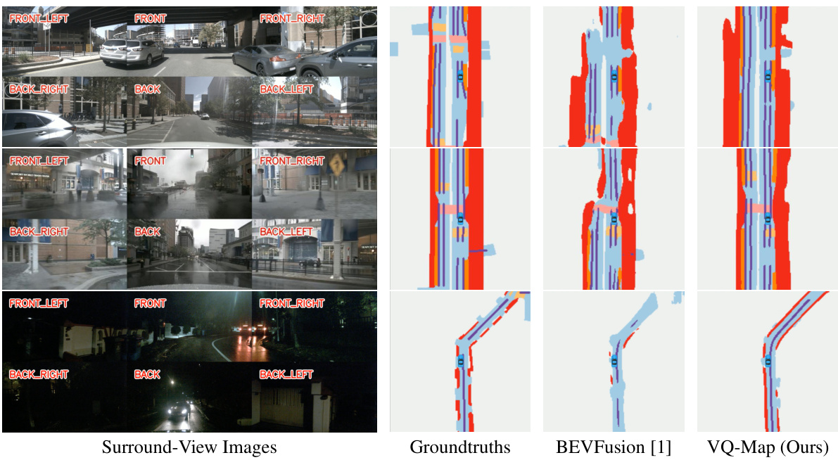
In this image, you can see:

• The raw camera feeds under different conditions (day, rain, night).
• The ground truth BEV map, which is the target for our VQ-VAE to learn to reconstruct.
• The output of the VQ-Map model. This output is generated by a decoder from the discrete tokens that were predicted. The high fidelity of the reconstruction demonstrates that the discrete tokens have successfully captured the essential semantic and geometric information of the scene.

Conclusion

In this lesson, we bridged the gap between continuous sensor perception and discrete generative modeling. You saw how the theoretical VQ-VAE architecture from our previous lesson becomes a practical and powerful tool for tokenizing the complex visual world in autonomous driving.

Key Takeaways:

• BEV as a Unified Space: Bird's Eye View provides a top-down grid representation that is essential for fusing data from multiple sensors with different perspectives.
• Creating the BEV Feature Map: Continuous BEV feature maps are created from camera images through a "lift-splat" process, which involves predicting depth, projecting 2D pixels into a 3D point cloud, and aggregating those points into a 2D grid.
• VQ-VAE as the Tokenizer: The VQ-VAE takes this continuous BEV feature map as input, processes it through an encoder, and uses a learned codebook to quantize it into a grid of discrete integer indices.
• Scene Tokens: These indices are the scene tokens, where each token represents a high-level semantic concept about a patch of the environment (e.g., lane, crosswalk, road boundary). This discrete representation is exactly what a Transformer-based planner needs.

Preview of the Next Lesson:

We have now successfully tokenized the environment. However, a planner must also reason about its own actions. In the next lesson, "Deep Dive: DAP (Discrete-token Autoregressive Planner)," we will explore the complete DAP architecture. You will learn how it also tokenizes the ego-vehicle's trajectory and navigation commands, and how it uses a unique autoregressive interleaving strategy to predict both the world's evolution and its own path within a single, unified sequence.