Sparse Activation for Efficient Model Scaling

Introduction

In the previous modules, we've built a comprehensive understanding of the Transformer architecture. We saw that a Transformer block has two main computational hubs: the self-attention mechanism and the Feed-Forward Network (FFN). In our last lesson, we focused on making attention efficient, culminating in our analysis of Multi-head Latent Attention (MLA), which brilliantly solves the KV cache memory bottleneck.

Now, we turn our attention to the other half of the block: the FFN layers. In a standard, or "dense," model, the FFN layers account for a significant portion of the total parameters. As we make models larger to increase their knowledge and capabilities, these FFN layers become a major source of computational cost, because every single parameter in the FFN is used to process every single token.

This lesson introduces a powerful paradigm to overcome this limitation: Mixture-of-Experts (MoE). Your learning outcome is to explain conditional computation and how sparse activation allows scaling model parameters without a proportional compute cost. We will explore how MoE enables the creation of models with hundreds of billions, or even trillions, of parameters while keeping the computational cost for inference manageable.

1. The Problem with Density: Why Scaling is Expensive

Imagine a large corporation where every single request, no matter how simple or specialized, must be processed by every single employee in every department. An accounting question would go through engineering, a legal query through marketing, and so on. This is incredibly inefficient.

This is precisely how a standard "dense" Transformer model works. For each token that enters an FFN layer, all the neurons (parameters) in that layer perform a calculation. This means the computational cost (measured in Floating Point Operations, or FLOPs) scales directly with the number of parameters. Doubling the size of the FFN layers doubles the compute. This makes scaling to massive parameter counts computationally prohibitive.

The solution is to work smarter, not harder. What if the corporation had a skilled receptionist who could route each request only to the one or two specialist departments best equipped to handle it? This is the core idea behind MoE.

This principle is called conditional computation: the computation performed is conditional on the input. Instead of activating the entire network, we only activate a small, relevant fraction of it. This is also known as sparse activation.

The following video provides an excellent visual introduction, contrasting a dense model with a sparse MoE model.

2. How MoE Implements Sparse Activation

As you just saw, the MoE architecture implements conditional computation by modifying the FFN layers. Instead of one large FFN, an MoE layer consists of two key components.

To formalize this, please read the first two sections of the following blog post from Hugging Face, which provides a concise and clear explanation.

From the reading, you've learned that an MoE layer is composed of:

1. Experts: A set of smaller, parallel neural networks. In the context of Transformers, each expert is typically its own FFN. You can think of these as the specialized "departments" from our analogy.
2. Router (or Gating Network): A small neural network that examines each incoming token and decides which expert(s) are best suited to process it. This is our "receptionist."

This architecture allows for sparse activation because for any given token, the router selects only a small number of experts (e.g., 2 out of 8, or 4 out of 64), while all other experts remain inactive and consume no computational resources.

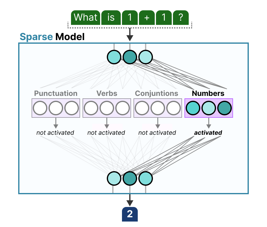
3. Scaling Parameters vs. Scaling Compute

The genius of MoE lies in its ability to decouple the growth of model parameters from the growth of computational cost. This introduces two important concepts:

• Total Parameters: The sum of all parameters in the model, including all experts. This number can be massive (e.g., the 1.8 trillion parameters rumored for GPT-4). The total parameter count determines the model's knowledge capacity and the amount of VRAM needed to load it.
• Active Parameters: The number of parameters actually used during inference for a single token. This includes the shared components of the model (like attention layers) plus the small number of experts selected by the router. This much smaller number determines the actual computational cost (FLOPs) and, therefore, the inference speed.

The Mixtral 8x7B model is a famous real-world example of this principle. The following video clip explains its architecture and clearly distinguishes between its total and active parameters.

As the video explains, a model like Mixtral 8x7B has a total of ~47 billion parameters. However, at any given step, it only uses ~13 billion active parameters. This means it has the knowledge capacity of a 47B parameter model but the inference speed and computational cost of a much smaller 13B parameter model.

This is the power of sparse activation: you get the benefits of a massive model (more knowledge, better performance) without the crippling computational cost of a dense equivalent.

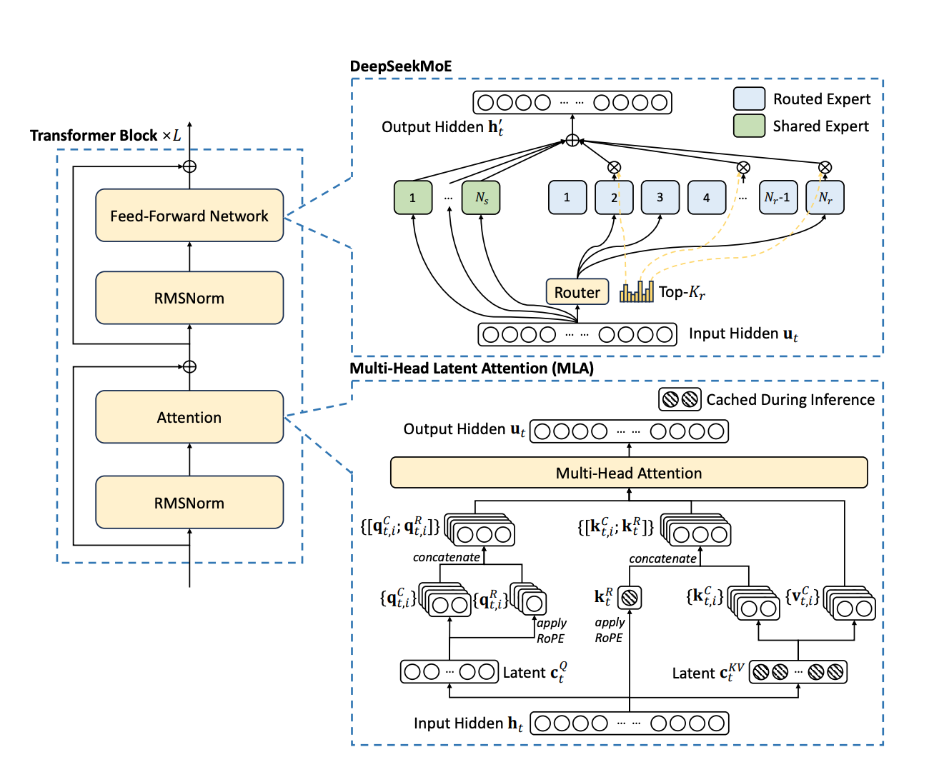
Finally, let's see how this all fits into the Transformer block architecture we know. The diagram below is from DeepSeek-V3, a model that heavily utilizes MoE.

Conclusion

In this lesson, we have explored the fundamental concepts behind Mixture-of-Experts.

Key Takeaways:

• Conditional Computation: Is the principle of activating only a subset of a model's parameters based on the specific input, rather than activating the entire network.
• Sparse Activation: Is the mechanism used to achieve conditional computation. In MoE, this is done by replacing dense FFN layers with a collection of specialized experts and a router that selects which ones to use for each token.
• Decoupled Scaling: MoE allows a model's total parameters (its knowledge) to scale massively while keeping the active parameters (its computational cost) manageable. This results in models that are both powerful and efficient at inference.

Preview of the Next Lesson:

We have answered the "what" and "why" of sparse activation. The next logical question is "how?" How does the router learn to make intelligent decisions? How are the experts structured? In our next lesson, we will dive deeper into the architecture of the MoE layer, describing the router network and the parallel expert FFNs in more detail.