Projection Matrices in Multi-Head Attention

Introduction

In our previous lesson, we explored the concept of multi-head attention, understanding that it allows a model to analyze a sentence from multiple perspectives simultaneously, like a team of specialists. We saw how different heads can learn to focus on different relationships (e.g., syntactic vs. semantic).

Today, we will dive deeper into the "how." The central question is: what mechanism enables each attention head to learn its own unique perspective? The answer lies in a set of trainable weight matrices.

Our learning goal for this lesson is to explain the role of the learned projection matrices $W_Q$, $W_K$, $W_V$, and $W_O$ in multi-head attention. These matrices are the core learnable parameters that empower the attention mechanism. Understanding their function is fundamental to grasping how Transformers learn to process language.

1. The Core Idea: Projecting to Specialized Subspaces

An input embedding for a word (e.g., "it") contains a rich, but jumbled, set of information about its meaning and context. To effectively calculate attention, we need to compare words based on specific roles they play in a given moment. The attention mechanism defines three such roles:

• Query (Q): Represents the current word's perspective, asking "What am I looking for?"
• Key (K): Represents a word's properties or what it "offers." It answers the Query's question by saying, "This is what I have."
• Value (V): Represents the content of a word. Once a Query finds a relevant Key, the associated Value is what's actually passed along.

The model creates these specialized Query, Key, and Value vectors by "projecting" the original input embedding into different vector spaces. These projections are performed by three distinct, learnable weight matrices: $W_Q$, $W_K$, and $W_V$.

Let's start with a great visual explanation.

As the article illustrates, each projection is a simple matrix multiplication. If we represent our input embeddings as a matrix $X$, the process looks like this:

But why do we need these different spaces? Why not just use the original embeddings? The following video explains the distinct purpose of the "similarity space" (created by Q and K) and the "content space" (created by V).

To summarize the key insight from the video:

• The Query and Key projections ($W_Q,W_K$) learn to create representations where the dot product is a meaningful measure of similarity for the attention task.
• The Value projection ($W_V$) learns to create representations that are most useful for the model's ultimate goal, which is constructing the final output embedding for the next layer.

2. Projections in Multi-Head Attention

Now, let's extend this to multi-head attention. As we learned last time, the goal is to have multiple heads learning different relationships in parallel. This is achieved by giving each attention head its own independent set of projection matrices.

If a model has $h=8$ attention heads, it will have 8 separate $W_Q$ matrices, 8 separate $W_K$ matrices, and 8 separate $W_V$ matrices.

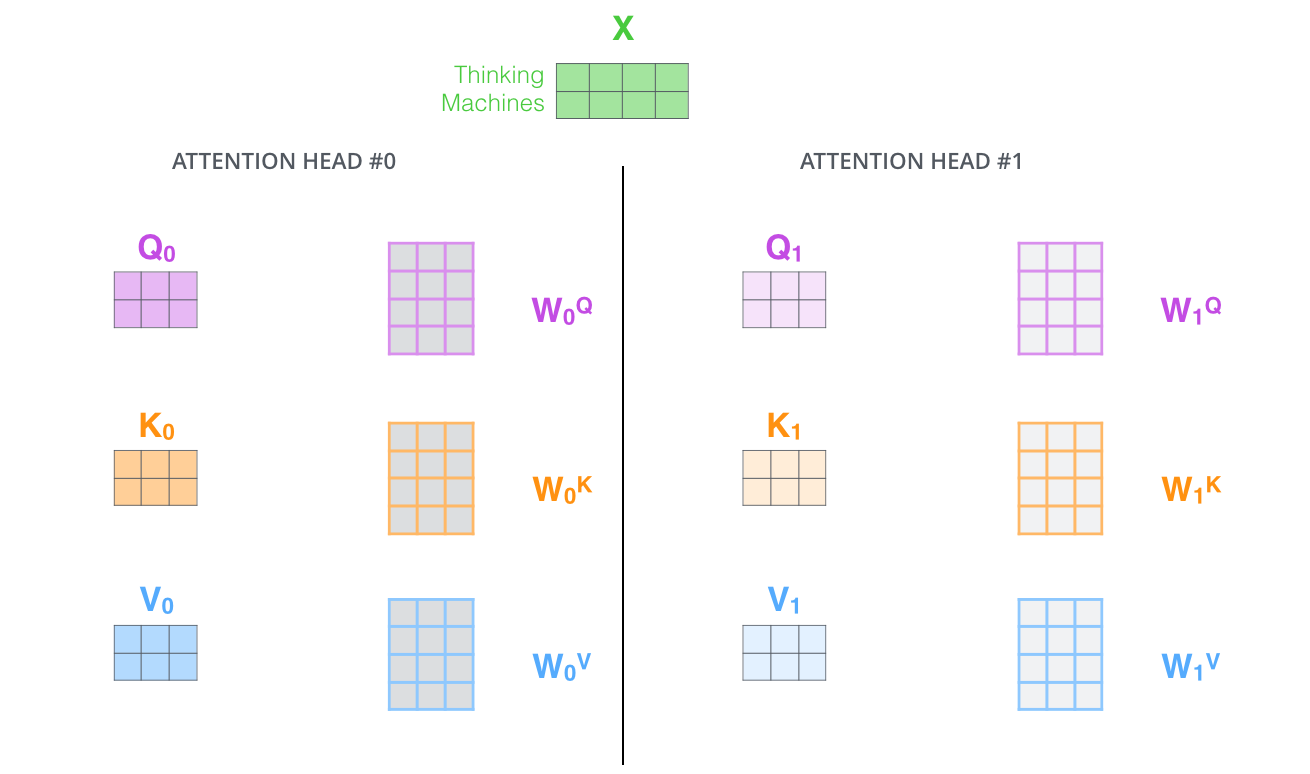
Because each head's weight matrices are initialized randomly and updated independently via backpropagation, they learn to project the input embeddings into different, specialized subspaces. One head might learn to project words into a space where syntactic similarities are highlighted, while another projects them into a space that captures semantic relationships.

The formal definition and dimensionality are laid out clearly in the following reading.

3. The Final Piece: The Output Projection Matrix $W_O$

After each of the $h$ heads has computed its attention output, we are left with $h$ different output vectors for each word in the sequence. The feed-forward layer that follows expects a single vector per word, not $h$ of them. This is where the final projection matrix, $W_O$, comes in.

The process is:

1. Concatenate: The output vectors from all $h$ heads are concatenated together. If each head produces a 64-dimensional vector and we have 8 heads, the concatenated vector will be $8\times 64=512$ dimensions.
2. Project with $W_O$: This large, concatenated vector is then multiplied by the output weight matrix $W_O$.

The role of $W_O$ is twofold:

• Dimensionality Management: It projects the concatenated vector back to the main d_model dimension (e.g., 512), ensuring the output of the multi-head attention block has the same shape as the input, ready for the next layer.
• Information Synthesis: Crucially, $W_O$ is a learned matrix. It learns the optimal way to combine the outputs from all the different attention heads. It can amplify the signals from heads that are providing useful information for a given word and diminish the noise from heads that are less relevant in that context. It effectively acts as a communication layer between the specialized heads.

This video segment shows this final concatenation and projection step.

Conclusion

In this lesson, we dissected the roles of the crucial learnable matrices in multi-head attention.

Key Takeaways:

• $W_Q,W_K,W_V$: These are learned projection matrices that transform the input embeddings into specialized representations for the Query, Key, and Value roles.
• Representation Subspaces: In multi-head attention, each head has its own independent set of $W_Q,W_K,W_V$ matrices. This allows each head to learn a unique "subspace," focusing on different types of features or relationships in the data.
• $W_O$: This is the learned output projection matrix. It takes the concatenated outputs from all attention heads and learns to mix them into a single, rich representation, projecting the result back to the model's standard dimension.

These four types of matrices are the trainable parameters that allow the attention mechanism to be so powerful and flexible. They are what the model learns during its training process.

Preview of the Next Lesson:
We have now examined all the key components of the attention mechanism. In the next lesson, we will move to Module 3, "Transformer Architecture and LLM Basics," where we will assemble the full Transformer block. We'll see how this multi-head attention layer we've just studied fits together with the feed-forward network, residual connections, and layer normalization to form the fundamental building block of models like GPT.