Scaled Dot-Product Attention Calculation

Introduction

In the previous module, we established a complete, albeit high-level, picture of how an autoregressive language model is trained. We treated the core of the model as a "black box" that takes in a sequence of token embeddings and outputs predictive scores (logits). We ended by discussing teacher forcing and masking, which ensure the model learns to predict the next token based only on past tokens.

Now, it's time to open that black box. This lesson introduces scaled dot-product attention, the fundamental computation that powers the Transformer architecture. This is the mechanism that allows a model to dynamically weigh the importance of different words in a sequence to understand the context.

Your learning goal for this lesson is to compute scaled dot-product attention given query, key, and value matrices. We will break down the famous attention formula, understand the role of each component, and walk through a concrete calculation.

1. The Core Idea: Attention as Contextual Similarity

At its heart, attention answers a simple question: "To predict the next word, which other words in the context are most important?"

Consider the sentence: "Jane is going to the cinema to watch a new ____". To predict the blank, a model should pay more attention to "cinema" and "watch" than to "Jane" or "is". This "paying attention" is achieved by calculating a similarity score between words.

In our vector space of embeddings, one of the most direct ways to measure similarity is the dot product. Vectors pointing in similar directions will have a large positive dot product, while orthogonal vectors will have a dot product of zero.

This first video provides a wonderful and intuitive explanation of how similarity scores (like dot product) form the basis of attention.

The key idea is that we can create a new, better representation for a word by blending it with other words in the sequence, weighted by their similarity scores.

2. From Embeddings to Queries, Keys, and Values

The model doesn't just use the raw input embeddings to calculate similarity. Instead, it learns to project the input embeddings into three distinct spaces, creating three new vectors for each token:

1. Query (q): Represents the current token's "search query" asking for relevant context. It's the active word looking for information.
2. Key (k): Represents a token's "label" or "indexed feature." It's what other queries are compared against.
3. Value (v): Represents the actual content or meaning of a token. This is the information that gets passed along if the token is deemed relevant.

These q, k, and v vectors are generated by multiplying the input embedding vector (x) by three separate weight matrices (W_q, W_k, W_v) that are learned during training.

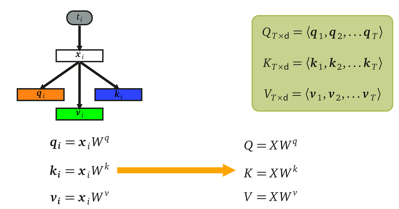
This projection gives the model flexibility. It can learn to transform the embeddings into a representation that is optimized for calculating similarity (via Q and K) and another representation that is optimized for conveying content (via V).

This next video explains this process clearly.

3. Computing Scaled Dot-Product Attention: The Formula

Now we have all the ingredients to assemble the full formula for scaled dot-product attention:

$\text{Attention}(Q,K,V)=\text{softmax}\left(\frac{Q{K}^T}{\sqrt{d_k}}\right)V$

Let's compute this step-by-step.

Step 1: Compute Similarity Scores (QK^T)

First, we compute the matrix product of the Query matrix Q and the transpose of the Key matrix K^T. The resulting matrix contains the dot product of every query vector with every key vector. This gives us a matrix of raw, unnormalized attention scores. A high value at position (i, j) means that query i (token i) finds key j (token j) highly relevant.

Step 2: Scale (/ sqrt(d_k))

Next, we scale these scores by dividing by the square root of the dimension of the key vectors, d_k. This is a critical step for stabilizing training.

• The Problem: The dot product of two vectors grows with their dimension. For high-dimensional embeddings (e.g., d_k = 512), the dot products can become very large.
• The Effect: Large input values to the softmax function cause it to "saturate"—producing extremely small gradients. This is the classic vanishing gradient problem, which would stall learning.
• The Solution: By dividing by $\sqrt{d_k}$, we rescale the variance of the dot products back to approximately 1, keeping the inputs to softmax in a well-behaved range.

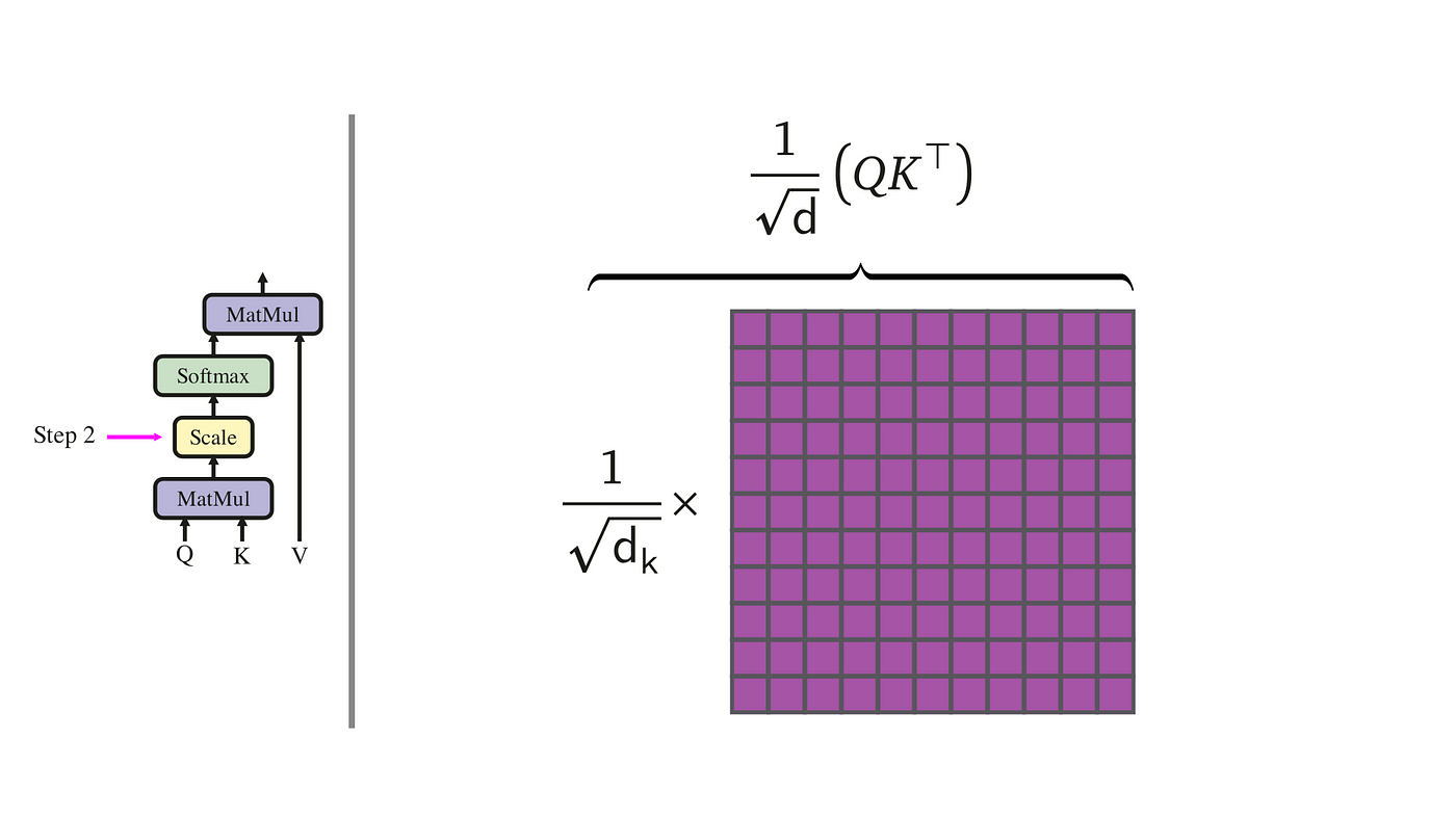
The following resources provide excellent explanations for this crucial step.

Step 3: Normalize with Softmax

We apply the softmax function row-wise to the scaled score matrix. This converts the scores into a probability distribution. Each row now represents the "attention weights" for a single query token, and the values in the row sum to 1.

Step 4: Produce the Output (...V)

Finally, we multiply the attention weights matrix by the Value matrix V. This computes a weighted sum. The output for each query token is a new vector that is a blend of all the value vectors in the sequence, weighted by their corresponding attention scores.

This final output vector is the new, context-aware representation for that token.

4. A Concrete Example: Computing Attention Step-by-Step

Now, let's put theory into practice by computing attention for a real sentence. The following blog post provides an excellent, code-based walkthrough. We will follow its steps to satisfy our learning objective.

By completing this walkthrough, you have successfully computed scaled dot-product attention! You started with input text and finished with a context-aware vector that incorporates information from the entire sequence based on learned attention weights.

Conclusion

In this lesson, you have opened the black box of the Transformer and mastered its core computational unit.

Key Takeaways:

• Attention creates context-aware representations by computing a weighted sum of all token values in a sequence.
• The weights are determined by the similarity between a token's Query vector and every other token's Key vector.
• The full computation is Attention(Q, K, V) = softmax( (QK^T) / sqrt(d_k) ) * V.
• The scaling factor 1/sqrt(d_k) is crucial for maintaining numerical stability during training by preventing the inputs to softmax from becoming too large.

Preview of the Next Lesson:
The mechanism we've just learned is powerful, but it looks at the sequence from only one "perspective." What if the model could benefit from calculating attention in different ways simultaneously? For example, one attention calculation could focus on syntactic relationships while another focuses on semantic ones. This is the idea behind multi-head attention, which we will explore in the next lesson. You'll see that it's simply a matter of running the scaled dot-product attention we learned today multiple times in parallel.