Graph Construction: Iterative Vector Insertion

From One Node to a Complete Graph

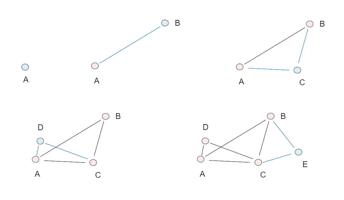
The strategy for building the entire NSW graph is elegantly simple. We start with an empty graph structure and iterate through every vector in our dataset, inserting them one by one using the nsw_insert function we designed previously.

1. The first vector added becomes the initial entry point.
2. The second vector is inserted by finding its nearest neighbors (just the first node) and connecting to it.
3. The third vector is inserted by searching from the entry point, finding its closest neighbors among the first two nodes, and connecting to them.
4. This process repeats for all N vectors in the dataset.

This iterative addition is the core of the construction process. The video segment below provides a clear, animated visualization of this exact procedure.

The image below provides a static, step-by-step view of this growth process. As each new node (B, C, D, E) is introduced, it forms connections to the nearest nodes already present.

The Emergence of Long-Range Links

A key question is why this simple iterative process creates an efficient graph. The nodes inserted early on are connected to neighbors that are, at that time, "close" but are far apart in the context of the final, dense graph. These early connections become the crucial long-range links that act as highways across the vector space, allowing the greedy search algorithm to traverse large distances in just a few hops. Later insertions create the dense, short-range links needed for fine-grained navigation in local neighborhoods.

The original NSW paper and many subsequent works are built on this principle. The construction process implicitly creates the multi-scale structure needed for efficient navigation.

A General Framework for Construction

Our approach fits into a well-established pattern for building proximity graphs. The flowchart below illustrates different methodologies. Our implementation aligns perfectly with diagram (b), the "NSWG-based approach."

For each vector, we loop through a process of:

1. Search: Find candidate neighbors for the new node (our nsw_search call).
2. Refinement (Prune/Connect): Establish connections and manage neighbor list sizes (the logic within nsw_insert).

This loop continues until all points are processed.

Implementation

With the nsw_insert function already defined, the implementation of the full build process is straightforward. We'll create a single function, nsw_build_graph, that contains the main loop.

#include <stdint.h>

// Forward declarations from previous lessons
typedef struct HNSWGraph HNSWGraph;
void nsw_insert(HNSWGraph* graph, uint32_t new_node_index, int M, int M_max, int ef_construction);

/**
 * @brief Builds the entire NSW graph by iteratively inserting all vectors.
 * 
 * This function iterates through all vectors loaded into the graph's memory
 * and calls nsw_insert for each one, effectively building the complete
 * search index.
 *
 * @param graph A pointer to the initialized HNSWGraph, with vector data loaded.
 * @param M The target number of neighbors for each new node.
 * @param M_max The maximum number of connections per node.
 * @param ef_construction The size of the candidate list for neighbor search during construction.
 */
void nsw_build_graph(
    HNSWGraph* graph,
    int M,
    int M_max,
    int ef_construction
) {
    // We assume graph->vectors and graph->current_size are already populated.
    // We also assume the graph->nodes array has been allocated.
    
    // Set the first node as the entry point if the graph is not empty.
    if (graph->current_size > 0) {
        graph->entry_point_node = 0;
        // The first node (index 0) has no neighbors to connect to yet.
        // The loop starts from the second node.
    } else {
        // Nothing to do for an empty graph
        return;
    }

    // Iteratively insert each subsequent vector into the graph.
    // Note: In a production system, you might add progress reporting here.
    for (uint32_t i = 1; i < graph->current_size; ++i) {
        nsw_insert(graph, i, M, M_max, ef_construction);
    }
}

This code demonstrates the power of modular design. The complexity of searching, finding neighbors, and managing connections is encapsulated within nsw_insert. The top-level build function becomes a simple, clean loop that clearly expresses the iterative construction algorithm. This entire process is a practical implementation of the ideas described in the foundational literature.

Conclusion

In this lesson, we completed our implementation of the Navigable Small World algorithm. By creating a main loop to call our nsw_insert function for every vector in the dataset, we now have a complete indexing pipeline. We can take a large set of raw vectors and transform it into a sophisticated graph data structure optimized for fast approximate nearest neighbor search.

Key Takeaways:

• Iterative Construction: The NSW graph is built by sequentially inserting each vector from the dataset.
• Emergent Structure: The desirable "small-world" properties, including a mix of long-range and short-range links, emerge naturally from this simple, iterative process.
• Modular Implementation: The complex logic of single-node insertion is encapsulated in its own function, allowing the main build process to be implemented as a simple and understandable loop.
• Efficient Scaling: The construction complexity of $O(N\log N)$ makes this a practical and powerful technique for the high-performance system we are building.

We now have two distinct methods for finding nearest neighbors: the brute-force sequential scan from Module 4 and our new, far more complex NSW graph search. Is the complexity worth it? In the next lesson, we will answer that question by benchmarking the search speed and recall of our NSW implementation against the exact k-NN search baseline. This will allow us to quantitatively measure the performance trade-offs and validate the effectiveness of our ANN index.