Connection Pruning for Maximum Node Connections

From Simple Eviction to Robust Re-selection

In the previous lesson, our logic for handling a full neighbor list was:

1. Find the most distant neighbor currently connected to node n.
2. Compare its distance to the distance of the new node q.
3. If q is closer, swap it with the most distant neighbor.

This is a reasonable greedy approach, but it has a subtle flaw. It only considers distance, not the spatial distribution or "diversity" of neighbors. A node's connections are its window to the rest of the graph; a diverse set of connections pointing in different directions allows for much more efficient long-range traversal during a search. Our simple eviction method might inadvertently create a cluster of very close neighbors, sacrificing a valuable long-range link.

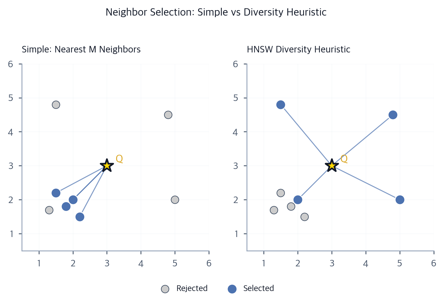
The original HNSW paper proposes a more robust method. Instead of a simple swap, it treats pruning as a re-selection process. The algorithm is as follows:

1. A new node q is to be connected to an existing neighbor n.
2. We tentatively add q to n's connection list. The list now temporarily has M_max + 1 connections.
3. We then run our powerful SELECT-NEIGHBORS algorithm on this oversized list of M_max + 1 candidates.
4. The algorithm selects the best M_max neighbors from this pool.
5. Node n's connection list is replaced with this new, optimal set of M_max neighbors.

This approach is superior because it allows us to reuse the same sophisticated logic (e.g., the diversity heuristic) for maintaining graph health that we use for initial insertion.

The Canonical Pruning Algorithm

The official HNSW paper formalizes this exact process. Let's look at the pseudocode, as it provides a clear blueprint for our C implementation.

The pseudocode from the article "HNSW: Hierarchical Navigable Small World" also reinforces this idea by showing prune_connections as a separate, explicit step in the insertion process.

C Implementation Task: Refactoring hnsw_connect_neighbors

Your task is to refactor the hnsw_connect_neighbors function you wrote in the last lesson. Instead of the if/else block that treats the "full" and "not full" cases differently, you will implement the unified, more robust algorithm.

The new logic for handling each neighbor n will be:

1. Add: Unconditionally add the new_node_id to n's neighbor list for the current layer and increment its neighbor count.
2. Check: Check if n's neighbor count for that layer now exceeds its capacity (M_max or M_max0).
3. Prune: If it does, you must shrink its connection list back to the capacity. To do this:
   • Create a temporary candidate list containing all M_max + 1 of n's current neighbors.
   • Call your existing hnsw_select_neighbors_heuristic function (or the simple version) on this candidate list, requesting it to select M_max neighbors.
   • Replace n's neighbor list with the new, pruned list of M_max neighbors returned by the selection function.
   • Ensure the neighbor count is set back to M_max.

Here is the C function from the last lesson. Your task is to modify the logic inside the second loop (// Part 2) to implement the new pruning strategy. You will need to assume you have a hnsw_select_neighbors_heuristic function available, which you implemented in a prior lesson.

// Assume definitions for HNSW, HNSWNode, HNSWLayer, and helper functions
// hnsw_get_node, hnsw_distance, and hnsw_select_neighbors_heuristic exist.

void hnsw_connect_neighbors(HNSW* hnsw, int new_node_id, int* selected_neighbors, int neighbor_count, int layer_level, int dim) {
    HNSWNode* new_node = hnsw_get_node(hnsw, new_node_id);
    HNSWLayer* new_node_layer = &new_node->layers[layer_level];

    // Part 1: Connect the new node TO its selected neighbors. (No change here)
    new_node_layer->count = neighbor_count;
    for (int i = 0; i < neighbor_count; i++) {
        new_node_layer->neighbors[i] = selected_neighbors[i];
    }

    // Part 2: Connect each neighbor back TO the new node. (Refactor this part)
    for (int i = 0; i < neighbor_count; i++) {
        int neighbor_id = selected_neighbors[i];
        HNSWNode* neighbor_node = hnsw_get_node(hnsw, neighbor_id);
        HNSWLayer* neighbor_layer = &neighbor_node->layers[layer_level];

        // --- OLD LOGIC TO BE REPLACED ---
        // if (neighbor_layer->count < neighbor_layer->capacity) { ... } 
        // else { ... simple eviction logic ... }
        // --- END OF OLD LOGIC ---

        // +++ NEW LOGIC GOES HERE +++
        // 1. Add new_node_id to neighbor_layer's list.
        // 2. Increment neighbor_layer->count.
        // 3. If neighbor_layer->count > neighbor_layer->capacity:
        //      a. Create a temporary array of all current neighbors.
        //      b. Call hnsw_select_neighbors_heuristic to get the best `capacity` neighbors.
        //      c. Update neighbor_layer->neighbors with the result.
        //      d. Set neighbor_layer->count = neighbor_layer->capacity.
    }
}

This refined implementation is a significant step toward a production-quality vector database. It ensures that the graph doesn't degrade over many insertions and that the structural invariants (M_max) that guarantee performance are strictly maintained.

Conclusion

In this lesson, we elevated our HNSW implementation by replacing a simple pruning heuristic with the formally correct and more robust algorithm from the foundational HNSW paper. This change, while subtle, has a significant impact on the long-term quality and performance of the search index. It's a perfect example of the level of detail required in high-performance systems engineering.

Key Takeaways:

• Pruning as Re-selection: The best practice for pruning is not to simply evict the "worst" node, but to re-run the neighbor selection algorithm on the oversized set of candidates.
• Component Reuse: A well-designed system reuses its core components. We now use hnsw_select_neighbors for both initial insertion and for graph maintenance during pruning.
• Maintaining Graph Quality: This robust pruning method actively maintains the diversity and quality of connections for all nodes in the graph, preventing performance degradation over time as more vectors are inserted.
• Enforcing Invariants: Pruning is the mechanism that strictly enforces the M_max and M_max0 connection limits, which are critical for predictable memory usage and search complexity.

You have now implemented all the core components of the HNSW insertion algorithm: probabilistic layer assignment, layer-by-layer searching, heuristic neighbor selection, and robust connection pruning. This concludes our deep dive into graph construction.

In the next module, "Concurrent Graph Operations," we will tackle a new challenge: how to build and search this graph using multiple threads. You'll apply your systems programming knowledge to implement thread pools, manage race conditions with locks, and explore lock-free techniques with atomic operations to maximize performance on modern multi-core CPUs.