Hello! In our last lesson, we explored regularization (L1 and L2), a key technique for preventing overfitting by penalizing model complexity. Now that we have a tool to control complexity, we need a way to diagnose whether our model has the right level of it. Is it too simple? Is it too complex? Or is it just right?
This lesson introduces learning curves, one of the most powerful diagnostic tools in a data scientist's arsenal. By plotting a model's performance against the amount of training data, learning curves provide a clear visual signature for underfitting (high bias) and overfitting (high variance). Your goal for this lesson is to learn how to interpret these curves to diagnose your model's behavior and make informed decisions about how to improve it.
1. The Intuition: Learning Like a Student
Before diving into the technical details, let's build an intuition for what learning curves represent. A machine learning model learning from data is a lot like a student studying for an exam.
This video from the channel Underfitted provides an excellent analogy to get started.
A Critical Skill People Learn Too LATE: Learning Curves In Machine Learning.
Watch "A Critical Skill People Learn Too LATE: Learning Curves In Machine Learning" to build a strong conceptual foundation.
Pay close attention to these parts: The School Analogy: Understand the parallel between a student's performance on practice questions vs. the final exam and a model's performance on training vs. testing data. Diagnosing Underfitting: See how a high error on the training data itself is a clear sign the model hasn't learned the material. Diagnosing Overfitting: Observe how a big difference between training and testing error indicates the model has memorized answers but can't generalize. The Well-Fit Model: See what the learning curves for an ideal model look like.
As the video explains, we track two primary metrics:
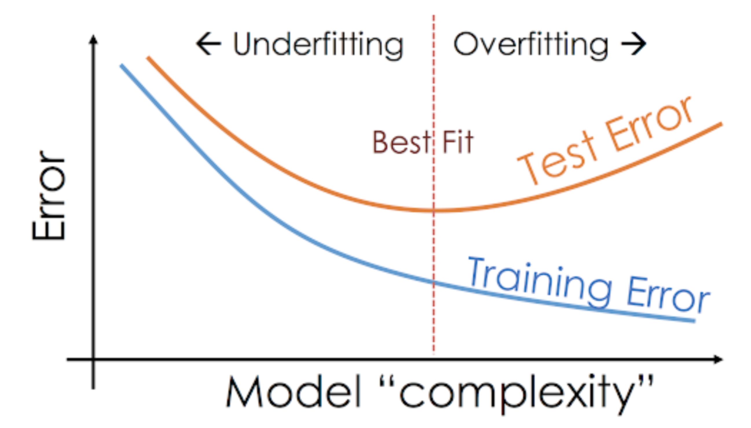
- Training Error: How well the model performs on the data it was trained on. This is like quizzing a student on the exact questions they studied. A high training error means the model is underfitting—it's too simple and hasn't even learned the basic patterns.
- Validation/Test Error: How well the model performs on new, unseen data. This is the real exam. A high validation error, especially when the training error is low, means the model is overfitting—it memorized the training data (noise included) but can't apply its knowledge to new problems.
2. Generating and Understanding Learning Curves
Learning curves plot these two error metrics not as a single number, but as a function of the training set size. This shows us how the model's learning and generalization ability evolve as it's exposed to more data.
Tutorial: Learning Curves for Machine Learning in Python for Data Science
The Dataquest article "Learning curves - the basic idea" provides a clear, step-by-step explanation of how these curves are constructed.
Focus on the text and the diagrams that show how the training and validation errors change as the number of training instances (n) increases from 1 to 50 to 100.
The process is as follows:
- Take a small subset of the training data (e.g., 10 instances).
- Train the model on this subset.
- Evaluate the model's error on both this small training subset and on a separate, held-out validation set.
- Increase the size of the training subset (e.g., to 50, 100, 500 instances...).
- Repeat steps 2 and 3 for each size.
- Plot the training errors and validation errors against the training set sizes.
The resulting plot reveals the model's learning dynamics and helps us connect its behavior back to the bias-variance tradeoff.
3. Interpreting the Three Classic Patterns
Now, let's learn to read the stories that learning curves tell. There are three main patterns you'll encounter. For this section, we'll continue with the excellent Dataquest tutorial, which provides clear examples.
Scenario 1: High Bias (Underfitting)
An underfit model is too simple to capture the underlying structure of the data. Its learning curves have a distinct signature.
Tutorial: Learning Curves for Machine Learning in Python for Data Science
This section from the Dataquest tutorial, "Learning curves - high bias and low variance," walks through an example using Linear Regression.
Read the section and pay close attention to the plot titled "Learning curves for a linear regression model". Notice how the training and validation errors behave.
Key Characteristics of an Underfit Model:
- High Training Error: The training error quickly plateaus at a high value. This is the smoking gun: the model performs poorly even on the data it was trained on.
- High Validation Error: The validation error also plateaus at a high value, very close to the training error.
- Small Gap: The gap between the training and validation curves is very small.
Diagnosis: The model is suffering from high bias. It's not complex enough to learn the data.
What to do? As the article notes, simply adding more training data will not help. Both curves have already converged. You need to increase model complexity. This could mean:
- Using a more powerful algorithm (e.g., moving from Linear Regression to a Random Forest).
- Engineering more informative features.
- Reducing regularization if you are using it too aggressively.
Scenario 2: High Variance (Overfitting)
An overfit model is too complex. It learns the training data, including the noise, so well that it fails to generalize to new data.
Tutorial: Learning Curves for Machine Learning in Python for Data Science
Now, let's look at the opposite case in the section "Learning curves - low bias and high variance," which uses a Random Forest Regressor.
Read this section and analyze the plot titled "Learning curves for a RandomForestRegressor model". Contrast its shape with the linear regression plot.
Key Characteristics of an Overfit Model:
- Low Training Error: The training error stays very low, and may not plateau at all. The model has no trouble memorizing the training data.
- High Validation Error: The validation error is significantly higher than the training error. It might plateau at a high value or continue to slowly decrease.
- Large Gap: There is a large and persistent gap between the training and validation curves. This gap represents the model's failure to generalize.
Diagnosis: The model is suffering from high variance. It's too sensitive to the specifics of the training data.
What to do? Here, you have several options:
- Gather more data: A large gap suggests the model could improve if it had more examples to learn from. The validation curve may eventually converge towards the training curve.
- Apply regularization: This is exactly what we covered in the last lesson! Add L1 or L2 regularization to penalize complexity and shrink the gap.
- Reduce model complexity: For example, you could prune a decision tree or use fewer features.
Visual Summary
The image below shows these two common problems side-by-side. It is a perfect reference to have on hand.

Scenario 3: The "Good Fit"
Ideally, we want a model that balances bias and variance. Its learning curve reflects this balance.
Key Characteristics of a Well-Fit Model:
- The training and validation error curves converge towards each other.
- They both plateau at a reasonably low error value.
- The gap between the final, converged error values is small.
This indicates that the model has learned the general patterns from the training data and can apply them successfully to new data.
Conclusion
You've now learned how to use learning curves as a diagnostic tool to understand your model's behavior. This is a far more insightful approach than just looking at a single accuracy or error score.
Key Takeaways:
- Learning curves plot model performance (error) against training set size for both the training and validation sets.
- Underfitting (High Bias) is diagnosed when both curves converge at a high error. The solution is to increase model complexity.
- Overfitting (High Variance) is diagnosed by a large gap between a low training error and a high validation error. Solutions include adding more data or applying regularization.
- A Well-Fit Model shows the two curves converging at a low error with a minimal gap.
In this lesson, we've discussed training and validation sets conceptually. In our next session, we will dive into the practical side of this process. We'll cover how to properly implement train-test-validation splits and introduce k-fold cross-validation, which are essential techniques for reliably evaluating your models and generating the robust learning curves we've analyzed today.