Real-World EDA: From Data to Insights

Welcome back! In our recent lessons, we've built a solid foundation in data manipulation with pandas, visualization with Seaborn and Matplotlib, and specialized techniques for time-series analysis. Now it's time to bring all these skills together.

This lesson focuses on Exploratory Data Analysis (EDA), the systematic process of investigating a dataset to discover patterns, spot anomalies, test hypotheses, and summarize its main characteristics. Think of it as detective work for data. Our goal is to conduct a full EDA on a real-world dataset, a process that will not only generate valuable insights but also form the basis of your second portfolio project.

The EDA Workflow: A Structured Approach

Before diving into code, it's helpful to have a mental map of the EDA process. While it's often iterative, a typical EDA follows these key stages:

Data Loading and Initial Inspection: Getting the data into a DataFrame and taking a first look.
Data Cleaning and Preparation: Handling inconsistencies, missing values, duplicates, and formatting issues.
Univariate Analysis: Understanding the characteristics of individual variables.
Bivariate and Multivariate Analysis: Exploring relationships between variables.
Asking and Answering Questions: Formulating specific questions and using the data to find answers.
Summarizing and Documenting: Communicating your findings in a clear, structured way.

We'll follow this workflow using a fantastic, detailed video walkthrough as our guide.

A Guided EDA: Analyzing Roller Coaster Data

We will use an end-to-end video tutorial from Kaggle Grandmaster Rob Mulla. It provides a practical, step-by-step demonstration of a full EDA on a fun and interesting dataset about roller coasters.

Exploratory Data Analysis with Pandas Python

The video "Exploratory Data Analysis with Pandas Python" will be our primary guide. The instructor's process is clear, methodical, and representative of a high-quality EDA.

We will break down the video into the logical steps of the EDA process. For each part, focus on why a particular step is being taken, not just the code itself.

1. Data Loading and Initial Inspection

The first step is always to load your data and get a high-level overview of its structure and content.

Watch the beginning of the video to see how to set up the environment and perform the initial data assessment.

Initial Setup & Inspection: Pay close attention to the sequence of commands:
- Importing necessary libraries (pandas, numpy, matplotlib, seaborn).
- Loading the data with pd.read_csv().
- Using .shape to see the dimensions (rows, columns).
- Using .head() to preview the first few rows.
- Using .columns to list all column names.
- Using .info() and .dtypes to check data types and non-null counts.
- Using .describe() to get a statistical summary of numerical columns.

2. Data Cleaning and Preparation

Raw data is rarely perfect. This stage involves transforming the data into a clean, usable format for analysis. It's often the most time-consuming part of a data science project.

Continue with the video to see a thorough data cleaning process.

Data Preparation: This is a critical section. Observe how the following tasks are handled:
- Column Subsetting: Selecting only the columns relevant to the analysis. This simplifies the DataFrame.
- Renaming Columns: Making column names consistent and easier to work with (e.g., removing spaces, standardizing capitalization).
- Data Type Conversion: Explicitly converting columns to the correct type, like using pd.to_datetime() for dates.
- Handling Missing Values: Using .isna().sum() to identify columns with missing data. The video doesn't impute them here, but it's an important step to be aware of.
- Handling Duplicates: Identifying and removing duplicate rows using .duplicated() and .drop_duplicates(), sometimes based on a subset of columns.

3. Univariate Analysis: Understanding Each Feature

Now that the data is clean, we can analyze each variable individually to understand its distribution and characteristics.

Univariate Analysis: Watch how the video explores single variables.
- Categorical/Discrete Data: Using .value_counts() to see the frequency of each category and creating a bar plot to visualize the top entries.
- Continuous Data: Using histograms (.plot(kind='hist')) and Kernel Density Estimate plots (.plot(kind='kde')) to visualize the distribution of numerical features like Speed.

4. Bivariate and Multivariate Analysis: Finding Relationships

This is where we start uncovering interesting connections between variables. How does the speed of a roller coaster relate to its height? Do newer coasters have different characteristics?

Feature Relationships: This section demonstrates several powerful visualization techniques.
- Scatter Plots: Used to visualize the relationship between two numerical variables (e.g., Speed vs. Height). Note the use of hue in Seaborn to add a third dimension (like Year_Introduced) to the plot.
- Pair Plots: seaborn.pairplot creates a matrix of scatter plots for all pairs of selected numerical features, giving a quick overview of all bivariate relationships.
- Correlation Heatmaps: A heatmap of the correlation matrix (.corr()) visually represents the linear relationships between all numerical variables. This is a key tool for spotting potential multicollinearity, a topic you've previously explored.

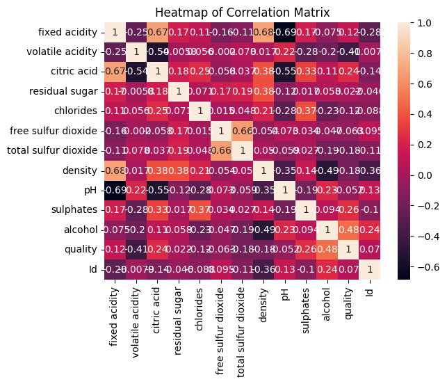
A correlation heatmap showing the relationships between different characteristics of wine. Red colors indicate a positive correlation, blue colors indicate a negative correlation, and the intensity of the color represents the strength of the relationship. This is a fundamental tool in EDA.

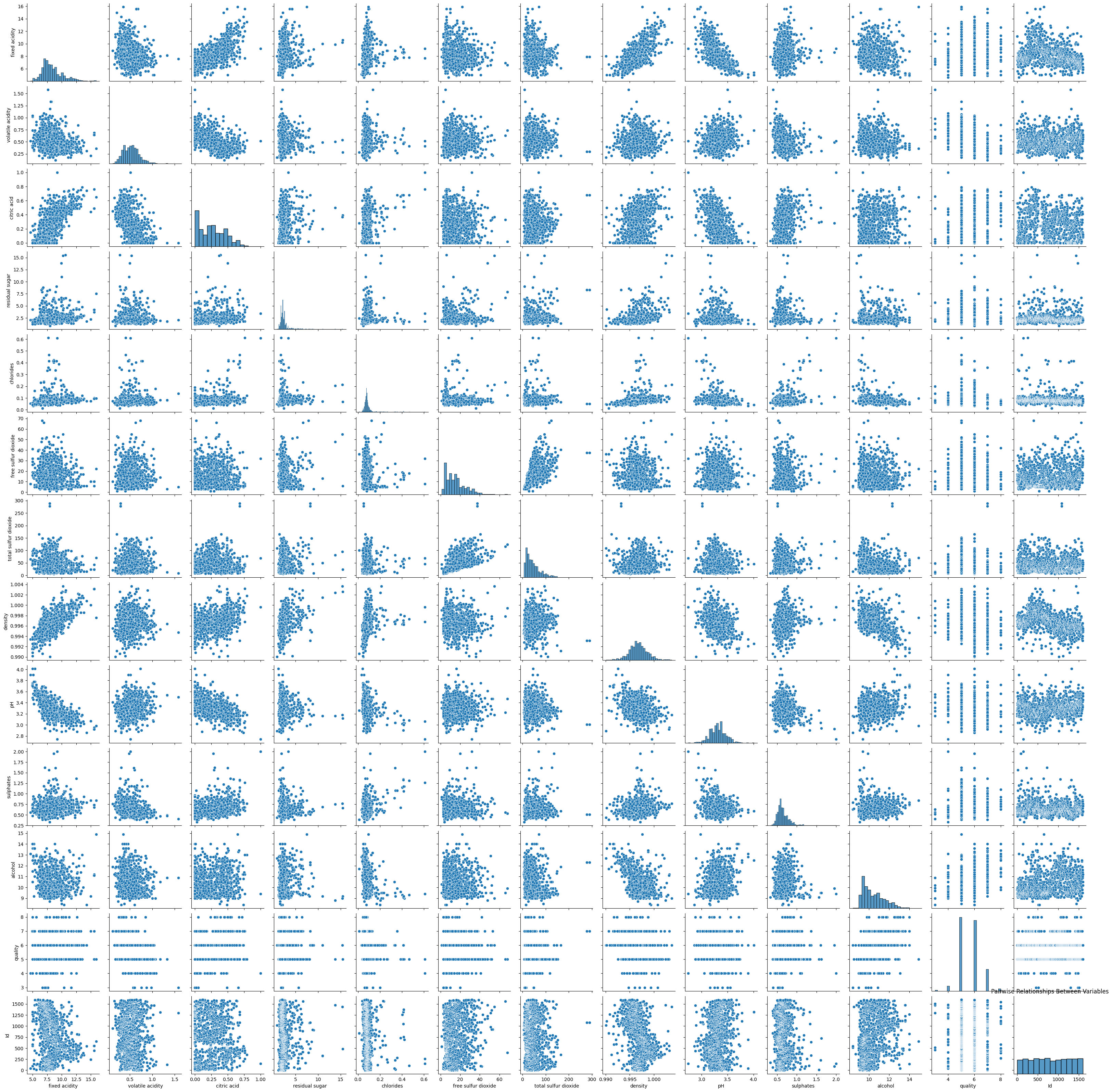
A pair plot showing scatter plots for pairs of variables and histograms for individual variables on the diagonal. This provides a comprehensive visual summary of relationships and distributions.

5. Asking and Answering Questions with Data

The ultimate goal of EDA is to generate insights. A great way to do this is to formulate specific questions and use your data analysis skills to answer them.

Answering a Question: The video ends by posing a question: "What are the locations with the fastest roller coasters (with a minimum of 10 coasters)?" Watch how a chain of pandas operations (.query(), .groupby(), .agg(), .sort_values()) is used to answer this question and visualize the result.

Adapting EDA for Time-Series Data

The roller coaster dataset included dates, but what if the temporal component is the central focus, like in the energy consumption data from our last lesson? For such datasets, we can enhance our EDA with specialized time-series techniques.

The previous lesson introduced you to resampling and rolling windows. Let's look at another resource that formalizes time-series EDA.

Time Series Forecasting: A Practical Guide to Exploratory ...

This article from Towards Data Science provides an excellent template for time-series EDA.

Please read the sections "3. Seasonal Plots" and "4. Box Plots". These sections show how to: Create seasonal plots to compare patterns across different years, weeks, or days. Use box plots grouped by time periods (e.g., month, day of the week, hour) to analyze the distribution and identify outliers within those periods. These techniques are powerful additions to your EDA toolkit, especially for datasets where seasonality and trends are important. For example, a seasonal plot could reveal that a company's sales always peak in December, while an hourly box plot might show that website traffic is most variable in the evenings. Documenting Your Findings: From Analysis to Story An EDA is only as valuable as your ability to communicate its findings. A well-documented Jupyter Notebook serves as both a record of your work and a compelling story for others (like potential employers). The key is to combine your code with clear explanations using Markdown cells. Explain what you're doing, why you're doing it, and what you've found.

These techniques are powerful additions to your EDA toolkit, especially for datasets where seasonality and trends are important. For example, a seasonal plot could reveal that a company's sales always peak in December, while an hourly box plot might show that website traffic is most variable in the evenings.

Documenting Your Findings: From Analysis to Story

An EDA is only as valuable as your ability to communicate its findings. A well-documented Jupyter Notebook serves as both a record of your work and a compelling story for others (like potential employers).

The key is to combine your code with clear explanations using Markdown cells. Explain what you're doing, why you're doing it, and what you've found.

Mastering Exploratory Data Analysis (EDA)

This article provides great advice on the final, and most important, part of EDA: turning your observations into a narrative.

Read the sections "Step 15: Observing Data, Insights, and Storytelling" and "Conclude your summary". Focus on the process of: Observation: Stating a factual pattern (e.g., "Sales spike in Q4"). Insight: Interpreting that pattern (e.g., "...possibly due to holiday shopping."). Storytelling: Weaving these insights into a coherent narrative that addresses a larger business question.

Conclusion

In this lesson, you've walked through the entire Exploratory Data Analysis workflow, from initial data loading to generating and communicating actionable insights. You saw how to apply the pandas and visualization skills from previous lessons in a structured, methodical way.

Key Takeaways:

EDA is a process: It's a systematic investigation involving cleaning, analyzing, and visualizing data to build understanding.
Start broad, then go deep: Begin with a high-level overview (.info(), .describe()) before diving into individual features (univariate) and then their relationships (bivariate/multivariate).
Visualize everything: Plots are your best tools for uncovering patterns, trends, and outliers. Use a variety of plots like histograms, box plots, scatter plots, and heatmaps.
Ask questions: The most valuable insights come from using the data to answer specific, well-defined questions.
Document as you go: A well-commented and documented analysis is a valuable asset for your portfolio.

In the next lesson, we will focus on translating this process into a polished Jupyter Notebook, which will become the second major project for your portfolio.

Recommended resources