Polynomial Features and Feature Interactions

1. The Limit of Linearity

Linear models are a fantastic starting point: they are fast, interpretable, and work well when the relationship between features and the target is, well, linear. But what happens when it's not?

Imagine trying to fit a straight line to data that follows a curve. The line will inevitably miss most of the points, leading to a model with high error (high bias). This is where polynomial regression comes in.

To build your intuition, let's start with a video that perfectly illustrates this problem.

The core idea is simple: if our data has a curve, we need a model that can curve, too.

2. Introducing Polynomial Features

How can we make a linear model produce a curve? The answer is surprisingly elegant: we don't change the model, we change the data we feed to it.

Polynomial regression is a form of linear regression where the relationship between the features and the target is modeled as an $n^{th}$ degree polynomial. Even though it models a non-linear relationship, it's considered a linear model because the regression function is linear in terms of the model's coefficients.

For a single feature $x$, a standard linear regression model looks like this:

For a 2nd-degree polynomial regression, we simply add a new feature, $x^2$, and fit the model to both $x$ and $x^2$:

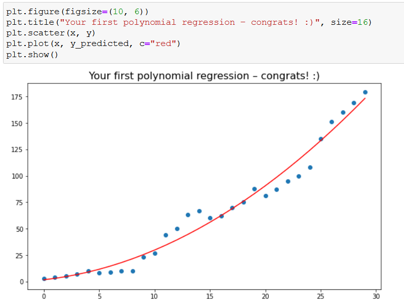
The model is still linear with respect to its coefficients (${\beta }_0,{\beta }_1,{\beta }_2$), but the function itself is a quadratic curve. Scikit-learn's PolynomialFeatures transformer automates the creation of these new features.

The following article provides a clear, step-by-step guide on how to implement this in Python.

3. Beyond Single Features: Interaction Terms

The power of PolynomialFeatures isn't limited to creating powers of single features. When you apply it to a dataset with multiple features (e.g., $x_1$ and $x_2$), it also generates interaction terms.

An interaction term is the product of two or more features (e.g., $x_1\times x_2$). It allows the model to learn relationships where the effect of one feature depends on the value of another.

For example, in a housing price model, the effect of having more bathrooms ($x_1$) on price ($y$) might be much greater for a large house (high square footage, $x_2$) than for a small one. The interaction term $x_1\times x_2$ helps the model capture this combined effect.

For two features $x_1,x_2$ and degree=2, PolynomialFeatures will generate the following set of features:

This includes the individual features, their squared terms, and the interaction term.

Let's continue with the same article, which has an excellent section on this.

For a more formal look at how these terms are generated, the resource "Polynomial Regression: Complete Guide" provides a clear mathematical breakdown under the heading "Multiple Variables" and the sub-heading "Example: Two Variables, Degree 2". You don't need to study it now, but it's a good reference (resource LINK).

4. Best Practices and The Danger of Overfitting

While powerful, polynomial features come with a major caveat: overfitting. As you increase the polynomial degree, the model becomes more flexible and can fit the training data more closely. However, a very high degree will cause the model to fit the noise in the data, not just the underlying signal. This leads to poor performance on new, unseen data.

Choosing the right degree is a classic bias-variance tradeoff.

• Low degree (e.g., 1): High bias, low variance (underfitting).
• High degree (e.g., 20): Low bias, high variance (overfitting).
• Just right: A balance that minimizes error on unseen data.

The video from NeuralNine has a fantastic segment that visualizes this exact problem.

Workflow with Pipelines

To avoid mistakes and keep your code clean, it's best practice to wrap your PolynomialFeatures transformer and your LinearRegression estimator in a scikit-learn Pipeline. This ensures the feature transformation is applied consistently during training, cross-validation, and prediction.

5. Hands-on Practice

Now it's your turn to apply these concepts. Let's use a synthetic dataset where the relationship is quadratic.

import numpy as np
import pandas as pd
import matplotlib.pyplot as plt
from sklearn.model_selection import train_test_split
from sklearn.linear_model import LinearRegression
from sklearn.preprocessing import PolynomialFeatures
from sklearn.pipeline import make_pipeline
from sklearn.metrics import r2_score




# 1. Generate synthetic data
np.random.seed(42)
X = 2 - 3 * np.random.normal(0, 1, 100)
y = X - 2 * (X ** 2) + 0.5 * (X ** 3) + np.random.normal(-3, 3, 100)




# Reshape X for scikit-learn
X = X[:, np.newaxis]




# 2. Split data
X_train, X_test, y_train, y_test = train_test_split(X, y, test_size=0.2, random_state=1)




# --- YOUR CODE GOES HERE ---




# 3. Fit a standard Linear Regression model
# Create and fit the model
linear_model = LinearRegression()
linear_model.fit(X_train, y_train)
y_pred_linear = linear_model.predict(X_test)
r2_linear = r2_score(y_test, y_pred_linear)
print(f"Linear Regression R^2: {r2_linear:.4f}")




# 4. Fit a Polynomial Regression model using a Pipeline
# Create and fit the pipeline (try degree=3, since the data was generated with a cubic function)
poly_model = make_pipeline(PolynomialFeatures(degree=3, include_bias=False), LinearRegression())
poly_model.fit(X_train, y_train)
y_pred_poly = poly_model.predict(X_test)
r2_poly = r2_score(y_test, y_pred_poly)
print(f"Polynomial Regression (degree=3) R^2: {r2_poly:.4f}")





# 5. Visualize the results
# Create a scatter plot of the test data
plt.figure(figsize=(10, 6))
plt.scatter(X_test, y_test, label="Actual Data")




# Plot the linear model's predictions
# Sort X_test to get a smooth line
X_test_sorted, y_pred_linear_sorted = zip(*sorted(zip(X_test, y_pred_linear)))
plt.plot(X_test_sorted, y_pred_linear_sorted, color='red', label=f'Linear Fit (R2={r2_linear:.2f})')




# Plot the polynomial model's predictions
X_test_sorted, y_pred_poly_sorted = zip(*sorted(zip(X_test, y_pred_poly)))
plt.plot(X_test_sorted, y_pred_poly_sorted, color='green', label=f'Polynomial Fit (R2={r2_poly:.2f})')

plt.title("Linear vs. Polynomial Regression")
plt.xlabel("Feature")
plt.ylabel("Target")
plt.legend()
plt.show()




# Optional challenge: Try fitting a model with degree=10 and see how the line changes.
# It will likely become very "wiggly" and overfit the training data.

Run this code and observe the results. You should see that the polynomial model has a much higher R² score and its prediction line fits the data far better than the simple linear model.

Conclusion

In this lesson, you've learned how to break the limits of linearity by automatically generating polynomial and interaction features. This technique adds significant power to your modeling toolkit, allowing you to capture complex patterns without immediately resorting to more opaque models.

Key Takeaways:

• Polynomial regression allows linear models to fit non-linear data by creating new features that are powers of the original features (e.g., $x^2,x^3$).
• When applied to multiple features, PolynomialFeatures also creates interaction terms (e.g., $x_1{x}_2$), which capture combined effects.
• The degree of the polynomial is a critical hyperparameter that controls model complexity. A high degree can easily lead to overfitting.
• Using a scikit-learn Pipeline to chain PolynomialFeatures and LinearRegression is the recommended best practice for a clean and robust workflow.

In our next lesson, we will shift our focus from creating features to addressing a common problem in classification tasks: handling imbalanced datasets. You'll learn techniques like SMOTE and class weighting to ensure your model performs well even when one class is much rarer than another.