Extracting Logic Levels from VTCs

1. What is a Voltage Transfer Characteristic (VTC)?

Imagine you have a digital device, like an inverter. You slowly sweep the input voltage ($V_{in}$) from low to high and, for each input value, you measure the resulting steady-state output voltage ($V_{out}$). If you plot $V_{out}$ on the y-axis against $V_{in}$ on the x-axis, the resulting curve is the device's Voltage Transfer Characteristic.

To get a feel for what a VTC looks like and how it's measured, let's watch a short video from MIT OpenCourseWare. It uses a buffer (output = input) as an initial example, but the principle of plotting $V_{out}$ vs. $V_{in}$ is identical for all combinational devices.

As the video shows, the VTC gives us a full picture of a device's static behavior. For an ideal inverter, the VTC would be a perfect step function: the output would be high for all inputs below a certain threshold and instantly switch to low for all inputs above it. However, real-world circuits don't switch instantly, which gives the VTC its characteristic 'S' shape.

2. Anatomy of a Realistic Inverter VTC

Now, let's dissect the VTC of a typical inverter to find our key logic levels. The image below shows a generic VTC with the important regions and points labeled.

As you can see, we can identify several key features on this graph:

• High and Low Output Levels ($V_{OH}$ and $V_{OL}$): These are the easiest to find. They correspond to the flat, "saturated" regions of the curve.

  • $V_{OH}$ is the output voltage when the input is a valid logic '0' (i.e., $V_{in}$ is low).
  • $V_{OL}$ is the output voltage when the input is a valid logic '1' (i.e., $V_{in}$ is high).
    In a well-designed CMOS inverter, these values are typically equal to the power supply voltage (VDD) and ground (GND), respectively.

• Input Logic Thresholds ($V_{IL}$ and $V_{IH}$): This is the most critical part of the analysis. $V_{IL}$ and $V_{IH}$ define the edges of the "forbidden" or "undefined" input region. They are formally defined as the points on the VTC where the gain ($g$), or the slope of the curve, is exactly -1.

  $$g=\frac{d{V}_{out}}{d{V}_{in}}=-1$$
  • $V_{IL}$: The input low voltage. It is the point on the upper part of the transition where the slope first reaches -1. For any input below $V_{IL}$, the device is guaranteed to see a '0'.
  • $V_{IH}$: The input high voltage. It is the point on the lower part of the transition where the slope once again reaches -1. For any input above $V_{IH}$, the device is guaranteed to see a '1'.

Why is the gain of -1 so important?
The region between $V_{IL}$ and $V_{IH}$ is the transition region, where the circuit acts like an amplifier (gain > 1). This high gain ensures a fast and sharp switch. Outside this region (gain < 1), the output is less sensitive to small changes in the input, which provides stability at the '0' and '1' logic states. The points where the gain is -1 are the conventional boundaries of this unstable transition region.

To see these definitions presented in the context of a real nMOS inverter, let's read a short section from a textbook on MOS devices.

3. Worked Example: Extracting Logic Levels

Now let's apply this knowledge. Your exam will likely present you with a VTC and ask you to extract these parameters. Let's work through a typical problem.

Consider the VTC for a logic inverter shown in the image below. We are asked to determine its DC characteristics.

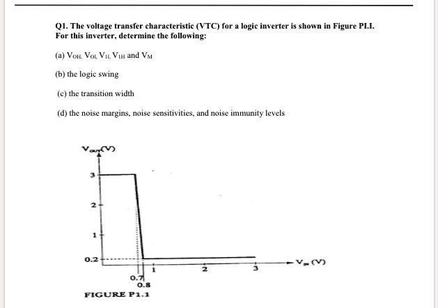
Let's find the logic levels step-by-step.

Step 1: Determine $V_{OH}$ and $V_{OL}$
These are the "flat" regions of the output voltage.

• By looking at the y-axis when $V_{in}$ is near 0, we can see the high output voltage is $V_{OH}=3.0V$.
• By looking at the y-axis when $V_{in}$ is high (e.g., at 3V), we see the low output voltage is $V_{OL}=0.2V$.

Step 2: Determine $V_{IL}$ and $V_{IH}$
These are the input voltages where the slope of the VTC is -1. In many textbook problems, these "knee" points of the curve are given or can be estimated as the boundaries of the sharp transition.

• From the graph, the output begins to drop sharply around $V_{in}=0.7V$. We will take this as $V_{IL}=0.7V$.
• The curve starts to flatten out into the low state after $V_{in}=0.8V$. We will take this as $V_{IH}=0.8V$.

Step 3: Calculate the Noise Margins
Now that we have all four parameters, we can calculate the noise margins using the formulas from our previous lesson.

• High Noise Margin ($N_M$_H): $$N_{MH}=V_{OH}-V_{IH}=3.0V-0.8V=2.2V$$
• Low Noise Margin ($N_M$_L): $$N_{ML}=V_{IL}-V_{OL}=0.7V-0.2V=0.5V$$

This inverter is significantly more robust against noise when its output is high than when it is low. This asymmetry is common in some logic families.

Step 4 (Bonus): Find the Switching Threshold ($V_M$)
The switching threshold ($V_M$) is the input voltage where $V_{out}=V_{in}$. We can estimate this by finding where the line $y=x$ would intersect the VTC. For this graph, it would be somewhere between 0.7V and 0.8V, likely around $V_M\approx 0.75V$.

Conclusion

In this lesson, you learned how to bridge the gap between the abstract concept of logic levels and the concrete behavior of a physical device. The VTC is a powerful tool that allows us to do just that.

Here are the key takeaways:

• The Voltage Transfer Characteristic (VTC) is a plot of $V_{out}$ vs. $V_{in}$ that graphically represents the static behavior of a digital gate.
• $V_{OH}$ and $V_{OL}$ can be read directly from the high and low flat portions of the VTC.
• $V_{IL}$ and $V_{IH}$ are formally defined as the input voltages where the slope of the VTC is -1. These points mark the boundaries of the high-gain transition region.
• By extracting these four levels from the graph, you can characterize a device and calculate its noise margins, giving you a quantitative measure of its robustness.

Preview of the Next Lesson

We calculated the noise margins in our example, but what do those numbers really mean for a circuit designer? In our next lesson, we will focus entirely on that question. We will calculate noise margins to determine the robustness of a digital circuit, exploring why large and symmetric noise margins are desirable and what happens when they are violated.