Gaussian Integral Evaluation

Introduction

Welcome back! In our last lesson, we established a firm grasp of complex numbers in their exponential form, a key piece of the mathematical language of quantum mechanics. You'll recall we previewed that our next step would be to tackle another essential tool: Gaussian integrals.

The Gaussian function, often called the "bell curve," is one of the most important functions in physics and probability theory. In quantum mechanics, it's used to model localized particles through wave packets. To ensure these wave packets represent a single particle, their corresponding probability distributions must integrate to 1—a process called normalization. This directly requires the evaluation of Gaussian integrals.

Today's learning outcome is to evaluate definite and indefinite Gaussian integrals using standard techniques. The challenge is that the function $e^{- x^{2}}$ has no simple antiderivative, so we can't solve its definite integral using the Fundamental Theorem of Calculus in the usual way. Instead, we will learn a brilliant trick involving multivariable calculus. We will then build on this result to solve more complex forms of Gaussian integrals that you will frequently encounter.

The Fundamental Gaussian Integral: A Classic Trick

The integral we want to solve is:

G = \int_{- \infty}^{\infty} e^{- x^{2}} d x

Since we cannot find an antiderivative for $e^{- x^{2}}$ , we'll use an ingenious method attributed to Poisson. The strategy involves squaring the integral, reinterpreting it as a volume, and then switching to a more convenient coordinate system.

To see this method in action, let's watch a clear, step-by-step walkthrough.

Gaussian Integration (Part 1)

This video, 'Gaussian Integration (Part 1)' from the channel Physics and Math Lectures, provides an excellent derivation of the fundamental Gaussian integral. It will guide us through the entire process.

Watch from timestamp 01:14 to 07:36. Pay close attention to these key steps: Squaring the integral and introducing a second integration variable, y. Combining the two integrals into a double integral over the entire xy-plane. Changing the coordinates from Cartesian (x, y) to polar (r, θ). Evaluating the now much simpler integral in polar coordinates.

Let's summarize the key steps from the video.

Square the Integral: We start by considering $G^{2}$ . Since the integration variable is a dummy variable, we can write:
$G^{2} = (\int_{- \infty}^{\infty} e^{- x^{2}} d x) (\int_{- \infty}^{\infty} e^{- y^{2}} d y)$
Form a Double Integral: We combine these into a double integral over the entire 2D Cartesian plane:
$G^{2} = \int_{- \infty}^{\infty} \int_{- \infty}^{\infty} e^{- (x^{2} + y^{2})} d x d y$
This integral represents the volume under the 2D Gaussian surface $z = e^{- (x^{2} + y^{2})}$ .
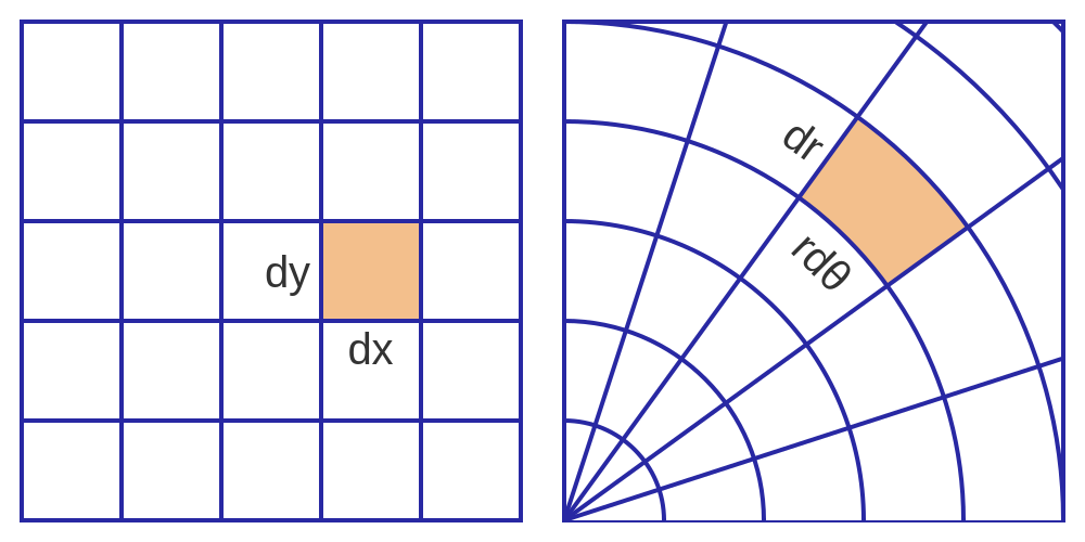
Switch to Polar Coordinates: The term $x^{2} + y^{2}$ suggests that polar coordinates would be a natural fit. We use the standard transformations:
- $x^{2} + y^{2} = r^{2}$
- The area element $d x d y$ becomes $r d r d θ$ .
- The limits of integration for the whole plane become $r \in [0, \infty)$ and $θ \in [0, 2 π]$ .

Differential Area Elements in Cartesian and Polar Coordinates — This image illustrates the transformation of the area element from $dx dy$ in Cartesian coordinates to the wedge-shaped $r dr d\theta$ in polar coordinates.

Evaluate the New Integral: The integral transforms into:
$G^{2} = \int_{0}^{2 π} \int_{0}^{\infty} e^{- r^{2}} r d r d θ$
This can be separated into two simpler integrals:
$G^{2} = (\int_{0}^{2 π} d θ) (\int_{0}^{\infty} r e^{- r^{2}} d r)$
The $θ$ integral is simply $2 π$ . The $r$ integral can be solved with a u-substitution (let $u = r^{2}$ , so $d u = 2 r d r$ ):
$\int_{0}^{\infty} r e^{- r^{2}} d r = \frac{1}{2} \int_{0}^{\infty} e^{- u} d u = \frac{1}{2} [- e^{- u}]_{0}^{\infty} = \frac{1}{2} (0 - (- 1)) = \frac{1}{2}$
Putting it all together: $G^{2} = 2 π \cdot \frac{1}{2} = π$ .
The Final Result: Since the integrand $e^{- x^{2}}$ is always positive, its integral $G$ must be positive. Therefore, we take the positive square root:
$\int_{- \infty}^{\infty} e^{- x^{2}} d x = π$

Generalization for $e^{- a x^{2}}$

A more general form that appears constantly in quantum mechanics is $\int_{- \infty}^{\infty} e^{- a x^{2}} d x$ for some positive constant $a$ . We can solve this with a simple change of variables. Let $u = a x$ , so $d u = a d x$ , or $d x = \frac{d u}{a}$ .

\int_{- \infty}^{\infty} e^{- a x^{2}} d x = \int_{- \infty}^{\infty} e^{- u^{2}} \frac{d u}{a} = \frac{1}{a} \int_{- \infty}^{\infty} e^{- u^{2}} d u = \frac{π}{a}

This is a fundamental result worth memorizing.

Test your understanding!

Evaluate the definite integral $\int_{- \infty}^{\infty} e^{- 5 x^{2}} d x$ .

Show answer

Using the formula $\int_{- \infty}^{\infty} e^{- a x^{2}} d x = \frac{π}{a}$ with $a = 5$ , we get:

\int_{- \infty}^{\infty} e^{- 5 x^{2}} d x = \frac{π}{5}

General Quadratic Exponents: Completing the Square

What if the exponent is a more general quadratic, like $- a x^{2} + b x + c$ ? This form is very common, for instance, when dealing with Gaussian wave packets that have an average momentum.

The standard technique here is completing the square. The goal is to manipulate the exponent into the form $- a (x - x_{0})^{2} + d$ , which we can then solve. For a more detailed look at this and other techniques, the following handout is a useful, concise reference.

QM Handout – Gaussian Integration

Let's consult the 'QM Handout – Gaussian Integration' from Durham University. It provides a compact summary of the key formulas and techniques.

Please read the section that begins 'For a general quadratic exponent...'. It's a short paragraph that demonstrates how completing the square reduces the problem to our known result.

As the resource shows, for an exponent $- a x^{2} + b x + c$ , we complete the square as follows:

- a x^{2} + b x + c = - a (x^{2} - \frac{b}{a} x) + c = - a (x - \frac{b}{2 a})^{2} + \frac{b ^{2}}{4 a} + c

So the integral becomes:

\int_{- \infty}^{\infty} e^{- a x^{2} + b x + c} d x = \int_{- \infty}^{\infty} e^{- a (x - \frac{b}{2 a})^{2} + \frac{b ^{2}}{4 a} + c} d x

We can pull the constant exponential term out of the integral:

= e^{\frac{b ^{2}}{4 a} + c} \int_{- \infty}^{\infty} e^{- a (x - \frac{b}{2 a})^{2}} d x

Now, we perform a change of variables: let $u = x - \frac{b}{2 a}$ , so $d u = d x$ . The integration limits remain from $- \infty$ to $\infty$ .

= e^{\frac{b ^{2}}{4 a} + c} \int_{- \infty}^{\infty} e^{- a u^{2}} d u

We've now reduced this to our known integral! The final result is:

\int_{- \infty}^{\infty} e^{- a x^{2} + b x + c} d x = \frac{π}{a} e^{\frac{b ^{2}}{4 a} + c}

This powerful formula allows you to solve any definite Gaussian integral with a real quadratic exponent.

Test your understanding!

Evaluate the integral $\int_{- \infty}^{\infty} e^{- 3 x^{2} - 6 x - 3} d x$ .

Show answer

We use the formula $\frac{π}{a} e^{\frac{b ^{2}}{4 a} + c}$ with $a = 3$ , $b = - 6$ , and $c = - 3$ .

The factor outside the integral is:

e^{\frac{b ^{2}}{4 a} + c} = e^{\frac{( - 6 ) ^{2}}{4 ( 3 )} - 3} = e^{\frac{36}{12} - 3} = e^{3 - 3} = e^{0} = 1

The integral part is:

\frac{π}{a} = \frac{π}{3}

So the final answer is $\frac{π}{3}$ .

Alternatively, completing the square directly:
$- 3 x^{2} - 6 x - 3 = - 3 (x^{2} + 2 x) - 3 = - 3 (x + 1)^{2} + 3 - 3 = - 3 (x + 1)^{2}$ .
The integral becomes $\int_{- \infty}^{\infty} e^{- 3 (x + 1)^{2}} d x$ . Let $u = x + 1$ , $d u = d x$ .
This gives $\int_{- \infty}^{\infty} e^{- 3 u^{2}} d u = \frac{π}{3}$ .

Gaussian Integrals with Polynomial Factors

Finally, let's consider integrals of the form $\int_{- \infty}^{\infty} x^{n} e^{- a x^{2}} d x$ . These arise when calculating expectation values (average values) of physical quantities like position or momentum.

Case 1: Odd powers of $x$

This case is simple. If $n$ is an odd integer ( $1, 3, 5, ...$ ), the integrand $f (x) = x^{n} e^{- a x^{2}}$ is an odd function, meaning $f (- x) = - f (x)$ . When you integrate any odd function over a symmetric interval like $(- \infty, \infty)$ , the result is always zero.

\int_{- \infty}^{\infty} x^{2 n + 1} e^{- a x^{2}} d x = 0 for n \geq 0

Case 2: Even powers of $x$

For even $n$ , the integrand is an even function, and the integral is non-zero. A clever technique to solve this is to differentiate our known result with respect to the parameter $a$ .

Let's start with our base formula:

G (a) = \int_{- \infty}^{\infty} e^{- a x^{2}} d x = π a^{- 1/2}

Now, let's differentiate both sides with respect to $a$ . On the left, we can bring the derivative inside the integral (this is called Leibniz's rule or "differentiating under the integral sign"):

\frac{d G}{d a} = \int_{- \infty}^{\infty} \frac{\partial}{\partial a} (e^{- a x^{2}}) d x = \int_{- \infty}^{\infty} (- x^{2}) e^{- a x^{2}} d x = - \int_{- \infty}^{\infty} x^{2} e^{- a x^{2}} d x

On the right, we just differentiate the explicit function of $a$ :

\frac{d}{d a} (π a^{- 1/2}) = π (- \frac{1}{2} a^{- 3/2})

Equating the two gives:

- \int_{- \infty}^{\infty} x^{2} e^{- a x^{2}} d x = - \frac{π}{2} a^{- 3/2}

So, we find our first result for an even power:

\int_{- \infty}^{\infty} x^{2} e^{- a x^{2}} d x = \frac{1}{2 a} \frac{π}{a}

We can repeat this process to find the integral for $x^{4}$ , $x^{6}$ , and so on. The general formula is provided in the QM Handout resource we looked at earlier (Section 2, formula 1).

Conclusion

In this lesson, you've mastered the essential techniques for evaluating Gaussian integrals, a critical skill for your journey into quantum mechanics. You've learned that even when a function has no elementary antiderivative, we can still find its definite integral using clever mathematical strategies.

Key Takeaways:

The fundamental Gaussian integral is $\int_{- \infty}^{\infty} e^{- x^{2}} d x = π$ .
The most common method to derive this is the polar coordinate trick: squaring the integral and evaluating the resulting 2D integral in polar coordinates.
The generalized form is $\int_{- \infty}^{\infty} e^{- a x^{2}} d x = \frac{π}{a}$ for $a > 0$ .
For a general quadratic exponent $- a x^{2} + b x + c$ , the technique of completing the square reduces the integral to a known form.
For integrals involving polynomial factors $x^{n}$ , you can use symmetry arguments (for odd $n$ ) or differentiation with respect to a parameter (for even $n$ ).

In our next lesson, we will move on to Fourier transforms. You'll see immediately why today's lesson was so important. The Fourier transform of a Gaussian function is, remarkably, another Gaussian function. Proving this requires evaluating an integral of the form $\int_{- \infty}^{\infty} e^{- a x^{2}} e^{- ik x} d x$ . Using Euler's formula from our first lesson and the technique of completing the square you learned today, you are now perfectly equipped to tackle it.

Recommended resources