Expectation and Standard Deviation for Continuous Distributions

Introduction

Welcome to the final lesson in our "Mathematical Preliminaries" module. Having mastered complex numbers, Gaussian integrals, Fourier transforms, and second-order ODEs, you've built an impressive mathematical toolkit. Today, we'll add the last piece: the language of statistics used to describe probability distributions.

This lesson focuses on the learning outcome: Compute expectation values and standard deviations for continuous probability distributions. While this is a concept from probability theory, it is absolutely central to quantum mechanics. The outcome of any quantum measurement is probabilistic, and these statistical tools are how we predict and characterize the average result and the spread of possible outcomes.

You'll find that the main tool we use is integration, a skill you've been honing throughout this module. We will define what "average" and "spread" mean for a continuous distribution and then apply these ideas to the Gaussian distribution, bringing you one step closer to your goal of mastering the Gaussian wave packet.

From Discrete to Continuous Averages

In everyday life, an average is simple: sum the values and divide by the count. If some values appear more often than others, we compute a weighted average. For instance, if we have a population with ages distributed according to a probability $P (a)$ , the average age $⟨ a ⟩$ is:

⟨ a ⟩ = all ages a \sum a \cdot P (a)

For a continuous variable like position $x$ , described by a probability density function $p (x)$ , the idea is the same, but the sum becomes an integral. The probability of finding the value in an infinitesimal interval $d x$ around $x$ is $p (x) d x$ .

The expectation value of $x$ , denoted $⟨ x ⟩$ , is the weighted average of all possible values of $x$ .

⟨ x ⟩ = \int_{- \infty}^{\infty} x \cdot p (x) d x

This integral gives us the "center of mass" or mean of the probability distribution.

More generally, for any function $f (x)$ , its expectation value is:

⟨ f (x)⟩ = \int_{- \infty}^{\infty} f (x) \cdot p (x) d x

A particularly important case for our purposes is the expectation value of $x^{2}$ , which is $⟨ x^{2} ⟩ = \int_{- \infty}^{\infty} x^{2} p (x) d x$ .

Lecture 4: Expectations, Momentum, and Uncertainty

For a formal introduction to these concepts, please look over the following notes from MIT OpenCourseWare. They provide a clear transition from discrete to continuous variables, which mirrors our discussion.

Read the first page of this PDF. Focus on the definitions of average for discrete variables and how they translate into integral form for continuous variables like position, governed by a probability density p(x). Notice the definition of (\langle f(x) angle) and the normalization condition.

Variance and Standard Deviation: Quantifying the Spread

The expectation value tells us the average outcome, but it doesn't tell us how spread out the possible outcomes are. For that, we need the variance and standard deviation.

The variance, denoted $σ^{2}$ , is the expectation value of the squared deviation from the mean. It measures the average squared "distance" of a measurement from the average value.

σ^{2} = ⟨(x - ⟨ x ⟩)^{2} ⟩

While this definition is intuitive, a more practical formula for calculation is derived by expanding the square:

σ^{2} = ⟨ x^{2} - 2 x ⟨ x ⟩ + ⟨ x ⟩^{2} ⟩ = ⟨ x^{2} ⟩ - 2 ⟨ x ⟩ ⟨ x ⟩ + ⟨ x ⟩^{2}

This simplifies to the crucial formula:

σ^{2} = ⟨ x^{2} ⟩ - ⟨ x ⟩^{2}

The standard deviation, $σ$ , is simply the square root of the variance:

σ = ⟨ x^{2} ⟩ - ⟨ x ⟩^{2}

The standard deviation gives us a direct measure of the width or spread of the distribution. A small $σ$ means the outcomes are tightly clustered around the mean $⟨ x ⟩$ , while a large $σ$ indicates they are widely dispersed.

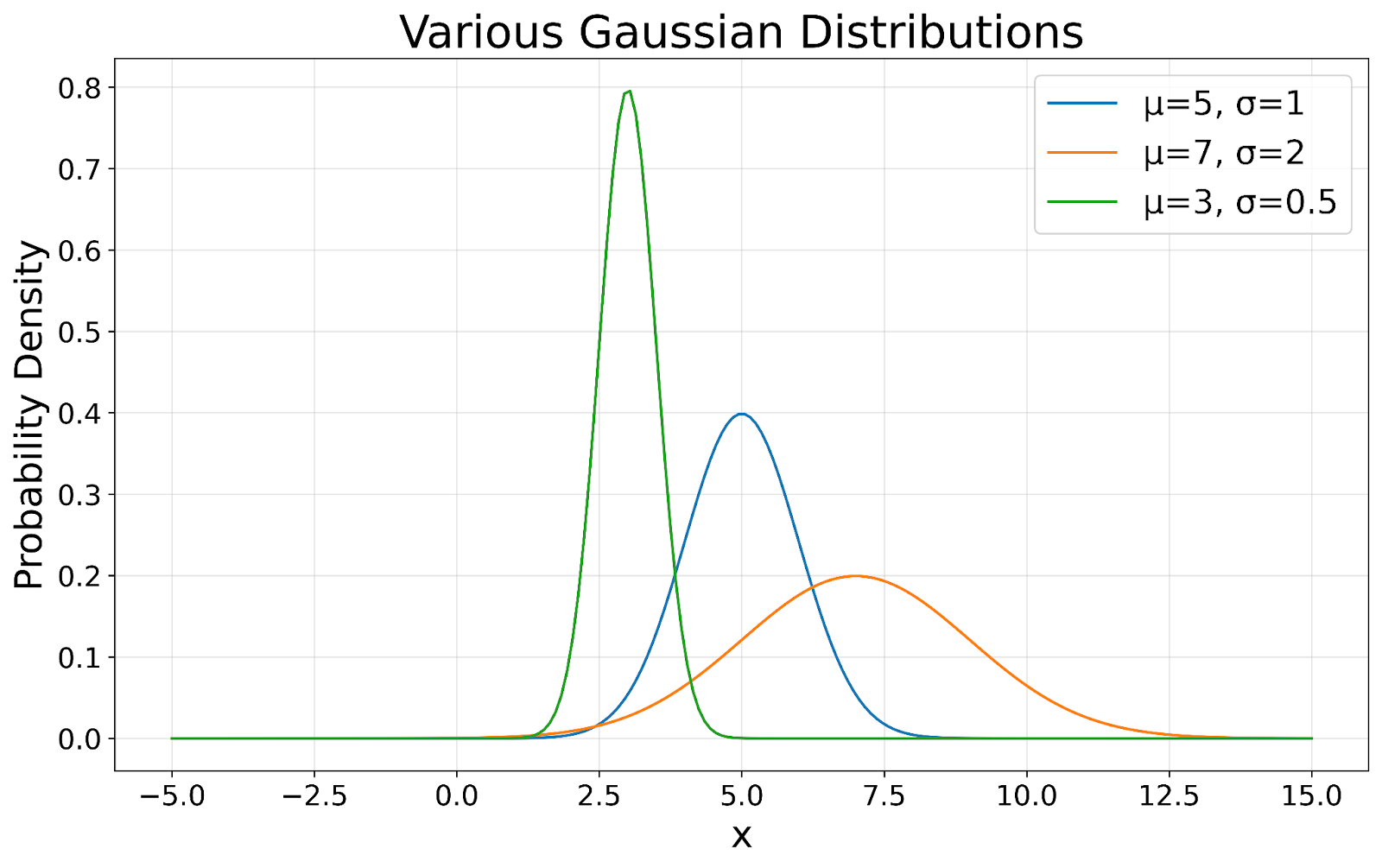
Comparison of Gaussian Distributions with Varying Mean and Standard Deviation — This image illustrates how the mean ($\mu$, equivalent to our $\langle x \rangle$) and standard deviation ($\sigma$) shape a Gaussian distribution. The mean sets the center of the peak, while the standard deviation controls its width. A larger $\sigma$ (orange curve) results in a wider, flatter curve, whereas a smaller $\sigma$ (green curve) leads to a narrower, taller curve.

A Complete Example: The Gaussian Distribution

Let's put all this together and analyze the Gaussian distribution, which is central to your goal. We will find its expectation value and standard deviation. The problem involves several integration techniques you've practiced, along with a few new powerful tricks.

We'll consider a general Gaussian probability density:

ρ (x) = A e^{- λ (x - a)^{2}}

where $A$ , $λ$ , and $a$ are positive real constants. Our task is to:

Find the normalization constant $A$ .
Calculate $⟨ x ⟩$ .
Calculate $⟨ x^{2} ⟩$ .
Compute the standard deviation $σ$ .

The following video provides a complete, step-by-step solution. We will go through it in segments.

Step 1: Normalization

First, we must ensure the total probability is 1. This is the normalization condition we've seen before, and it allows us to determine the constant $A$ .

Griffiths QM 1.6 Solution: Expectation Values For Gaussian Distribution (rho(x)=Ae^(-lambda(x-a)^2)

Let's begin by normalizing the Gaussian distribution. This process relies on the standard Gaussian integral you've already mastered.

Watch from the beginning to 5:41. Follow the steps to set up the normalization integral (\int ho(x) dx = 1) and solve for the constant A. Note the use of a change of variables to match the standard integral form.

Step 2: Calculating the Expectation Value $⟨ x ⟩$

Now that the distribution is normalized, we can calculate its mean. This part of the calculation introduces a very useful technique involving the symmetry of integrals.

Griffiths QM 1.6 Solution: Expectation Values For Gaussian Distribution (rho(x)=Ae^(-lambda(x-a)^2)

Next, we'll calculate the expectation value of x. Pay close attention to the argument made about integrating an odd function over a symmetric interval. This is a shortcut you will use frequently in quantum mechanics.

Watch from 5:41 to 10:06. Observe how the integral for (\langle x angle) is split into two parts after a change of variables. See how one integral is immediately identified as zero due to symmetry, greatly simplifying the calculation.

The result, $⟨ x ⟩ = a$ , should be intuitive: the Gaussian $e^{- λ (x - a)^{2}}$ is symmetrically peaked around $x = a$ , so its average value is naturally $a$ .

Step 3: Calculating $⟨ x^{2} ⟩$

This calculation is the most complex, but it demonstrates a powerful method known as "differentiation under the integral sign" or the "Feynman trick".

Griffiths QM 1.6 Solution: Expectation Values For Gaussian Distribution (rho(x)=Ae^(-lambda(x-a)^2)

Calculating (\langle x^2 angle) requires a more advanced approach. This segment introduces a clever trick: rewriting the integrand as the derivative of a simpler function with respect to a parameter.

Watch from 10:06 to 14:43. Focus on how the integral \int u^2 e^{-\lambda u^2} du is related to the derivative of the standard Gaussian integral with respect to \lambda. Don't worry if this technique is new; the video explains it clearly. This is a very elegant and powerful method for solving certain types of integrals.

Test your understanding!

Without re-watching the video, why did the middle integral in the expansion for $⟨ x^{2} ⟩$ (the one involving $2 a \int u e^{- λ u^{2}} d u$ ) immediately go to zero?

Show answer

The integrand, $u e^{- λ u^{2}}$ , is an odd function (since $u$ is odd and $e^{- λ u^{2}}$ is even). The integral is taken over a symmetric interval (from $- \infty$ to $\infty$ ). The integral of any odd function over a symmetric interval is always zero.

Step 4: Finding the Standard Deviation $σ$

Finally, we combine our results to find the standard deviation.

Griffiths QM 1.6 Solution: Expectation Values For Gaussian Distribution (rho(x)=Ae^(-lambda(x-a)^2)

With (\langle x angle) and (\langle x^2 angle) in hand, we can now easily compute the standard deviation.

Watch from 14:43 to 15:28. See how the results for (\langle x^2 angle) and (\langle x angle^2) are substituted into the formula (\sigma^2 = \langle x^2 angle - \langle x angle^2) to find the variance and then the standard deviation.

You have now calculated the mean ( $a$ ) and standard deviation ( $σ = 1/ 2 λ$ ) for a general Gaussian distribution, a result that will reappear when we study Gaussian wave packets in detail.

The Bridge to Quantum Mechanics

So, how does this connect to a quantum particle's wave function, $Ψ (x, t)$ ? According to Born's rule, one of the foundational postulates of quantum mechanics, the probability density for finding a particle at position $x$ at time $t$ is given by the squared modulus of its wave function:

p (x, t) = ∣Ψ (x, t) ∣^{2} = Ψ^{*} (x, t) Ψ (x, t)

With this rule, all the statistical tools we've just developed can be directly applied to the wave function to predict measurement outcomes.

Wavefunction Properties, Normalization, and Expectation Values

The following clip from Professor Dave Explains provides a concise explanation of how the statistical concept of an expectation value is used in quantum mechanics.

Watch from 15:10 to 18:16. Focus on the core idea: to find the expectation value of an observable (like position), you 'sandwich' its corresponding operator between \Psi^* and \Psi and integrate over all space.

Conclusion

This lesson concludes our survey of essential mathematical tools. You are now prepared to engage directly with the physics.

Key Takeaways:

The expectation value (or mean) of a continuous variable $x$ with probability density $p (x)$ is its weighted average: $⟨ x ⟩ = \int x p (x) d x$ .
The variance ( $σ^{2}$ ) and standard deviation ( $σ$ ) measure the spread of the distribution.
The most common formula for variance is $σ^{2} = ⟨ x^{2} ⟩ - ⟨ x ⟩^{2}$ .
In quantum mechanics, the probability density is given by Born's rule, $p (x) = ∣Ψ (x) ∣^{2}$ , allowing us to calculate the expected outcomes of measurements on a quantum system.
For a Gaussian distribution $p (x) \propto e^{- λ (x - a)^{2}}$ , the mean is $⟨ x ⟩ = a$ and the standard deviation is $σ = 1/ 2 λ$ .

You have officially completed the "Mathematical Preliminaries" module. Congratulations! You've built a strong foundation that will serve you well as we delve into the core principles of quantum mechanics.

Our next lesson marks the beginning of Module 2. We will finally introduce the time-dependent Schrödinger equation, the master equation that dictates how a quantum system's wave function evolves. We will dissect its components and begin to understand its profound implications.

Recommended resources

Introduction

From Discrete to Continuous Averages

Variance and Standard Deviation: Quantifying the Spread

A Complete Example: The Gaussian Distribution

Step 1: Normalization

Step 2: Calculating the Expectation Value ⟨x⟩

Step 3: Calculating ⟨x2⟩

Step 4: Finding the Standard Deviation σ

The Bridge to Quantum Mechanics

Conclusion

Step 2: Calculating the Expectation Value $⟨ x ⟩$

Step 3: Calculating $⟨ x^{2} ⟩$

Step 4: Finding the Standard Deviation $σ$