Dashboard Visual Design Principles

Why Good Design Matters

A well-designed dashboard does more than just look good. It communicates information clearly, guides your attention to what's most important, and helps you make better financial decisions at a glance. Your 5 years of experience in personal finance have given you a deep understanding of the key metrics; good design will make those metrics shine.

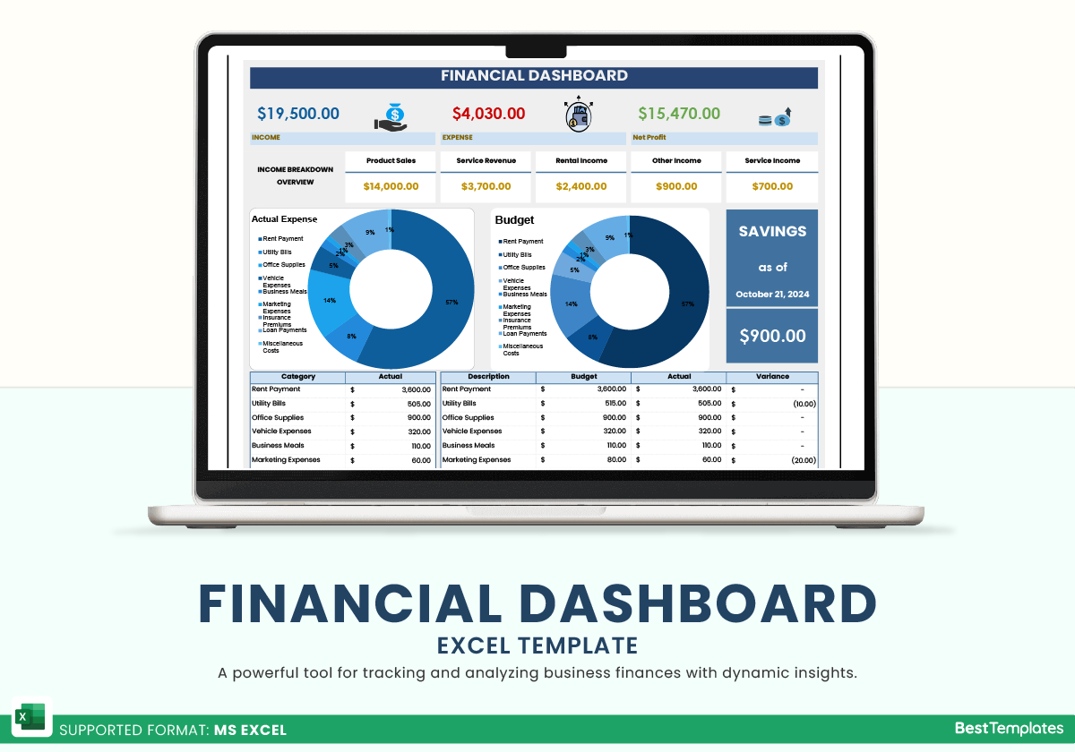
Let's look at an example of a clean, effective financial dashboard built in Excel.

Part 1: Core Principles of Effective Dashboard Design

Before we jump into Excel, let's cover a few fundamental principles that separate a great dashboard from a confusing one.

To summarize the key ideas from that reading and add a couple more:

• Visual Hierarchy: The most important information should be the most visually prominent. We achieve this through:

  • Position: People in Western cultures tend to read in a Z-pattern, so the top-left is prime real estate. This is where your most critical Key Performance Indicator (KPI), like Net Worth, should go.
  • Size & Scale: Larger elements draw more attention. Your main KPIs should be larger than secondary details.
  • The Inverted Pyramid: Place high-level summaries (KPIs) at the top, trends and comparisons in the middle, and granular details at the bottom.

• Layout & Whitespace: A clean, organized layout makes your dashboard trustworthy and easy to read.

  • Use a simple grid to align your charts and KPI boxes.
  • Use whitespace (empty space) to separate different sections. This is more effective than drawing lines everywhere.

• Color Strategy: Color should be used purposefully, not just for decoration.

  • Limited Palette: Stick to 2-3 main colors. A common strategy is to use neutral colors (like gray and white) for the background and structure, a primary "brand" color (like blue) for titles and accents, and reserved colors for signals (e.g., green for positive variance, red for negative).
  • Consistency: If "Income" is represented by blue in one chart, it should be blue in all charts. This reduces the mental effort required to understand the data.

• Simplicity (Avoiding "Chart Junk"): Every element on your dashboard should have a purpose. Remove anything that distracts from the data itself.

Part 2: Mocking Up Your Dashboard in Excel

Now, let's apply these principles by building the visual mock-up of your dashboard. We'll create the structure for your main KPIs.

Let's build this in your own Excel file.

1. Create and Prepare Your Dashboard Sheet:

   • Create a new worksheet and name it Dashboard.
   • Go to the View tab and uncheck Gridlines. This immediately makes the sheet look less like a spreadsheet and more like a canvas.
   • (Optional) Set a background color for the entire sheet. Select all cells (Ctrl+A) and choose a light, neutral fill color like a very light gray.

2. Create the Layout Structure:

   • As shown in the video, create a basic grid using column widths. A common technique is to have narrow columns for spacing and wider columns for content.
   • For example, make column A and column O narrow (e.g., width 2). Then make columns B through N a medium width (e.g., width 10). This creates a centered container for your dashboard.

3. Mock-Up Your First KPI Card:

   • We'll create a card for "Net Worth." Pick a block of cells, for example, B3:D6.
   • Title: Merge cells B3:D3. Type "Net Worth" and format it (e.g., Font: Segoe UI, Size: 14, Bold, Text Color: a dark blue). Center the text.
   • Value: Merge cells B4:D5. Type a placeholder value like $50,000. Format this to be the most prominent element (e.g., Font: Segoe UI Semibold, Size: 24). Center the text.
   • Variance/Comparison: Merge cells B6:D6. Type a placeholder like + $1,500 vs. last month. Format this to be smaller and lighter (e.g., Font Size: 10, Text Color: gray).
   • Borders & Fill: Select the entire block (B3:D6). Give it a white fill color and a light gray outline to make it look like a distinct card.

4. Replicate for Other KPIs:

   • Once you have a design you like, simply copy and paste this block of cells to create other KPI cards for metrics you want to track (e.g., Total Investments, Monthly Net Cash Flow, Savings Rate).
   • Place these cards along the top of your dashboard to follow the "inverted pyramid" principle.

Part 3: Advanced Formatting for a Professional Finish

To make your dashboard truly dynamic and easy to read, we can use some of Excel's powerful formatting features. We won't connect them to real data yet, but it's important to know how they work as we design.

Custom Number Formatting

This allows you to change how a number looks without changing its underlying value. It's perfect for adding symbols or text. For example, we can make positive numbers show an up arrow and negative numbers a down arrow.

The format string for this looks something like this: ▲ #,##0; ▼ #,##0; -
This tells Excel:

1. If the number is positive, show an up triangle and the number.
2. If the number is negative, show a down triangle and the number.
3. If the number is zero, show a dash.

Conditional Formatting

This is even more powerful. It automatically applies formatting (like cell color or font color) based on a rule. This is how you can make a negative cash flow value automatically turn red.

As you build your dashboard, think about where you can apply these rules. For example:

• The Net Cash Flow KPI value could turn red if it's negative.
• A Budget vs. Actual variance could turn red if you've overspent.

Conclusion

Congratulations! You've just designed the visual foundation of your personal finance dashboard. While it's just a static mock-up for now, you've made critical decisions about layout, hierarchy, and color that will make your final dashboard intuitive and powerful.

Key Takeaways:

• Design comes first: Mocking up the layout before adding data leads to a better end product.
• Follow core principles: A clear hierarchy, clean layout, purposeful color, and simplicity are key to effective dashboard design.
• Excel is a powerful design tool: By hiding gridlines, managing column widths, and using fill colors and borders, you can create a professional-looking interface.
• Advanced formatting adds dynamism: Custom Number Formatting and Conditional Formatting are essential tools for making your data communicate its meaning at a glance.

In our next module, "Tracking Expenses and Income," we'll start bringing this dashboard to life. We will begin by creating the detailed data entry tables for all your income and expense transactions and then write our first SUMIFS formulas to aggregate the data. These are the calculations that will eventually feed the beautiful KPI cards you designed today.