Evaluating Architectural Alternatives

From Business Goals to Engineering Targets: Defining Non-Functional Requirements (NFRs)

The criteria we use to judge an architecture are not arbitrary. They are the technical expression of business or product goals. These are often called non-functional requirements (NFRs) or quality attributes. As an architect, your first job is to listen to the business needs and translate them into a set of engineering characteristics that will guide your design.

For instance, a business stakeholder might say, "We need to get features out to customers faster." An architect translates this into concrete NFRs.

As the article shows, "fast time to market" isn't a single attribute. It decomposes into:

• Maintainability: How easy is it to find, fix, and change code?
• Testability: How easy and comprehensive is our testing?
• Deployability: How frequently, quickly, and safely can we deploy?

These NFRs now form the context for our trade-off analysis. Other common NFRs include performance, scalability, availability, security, and cost.

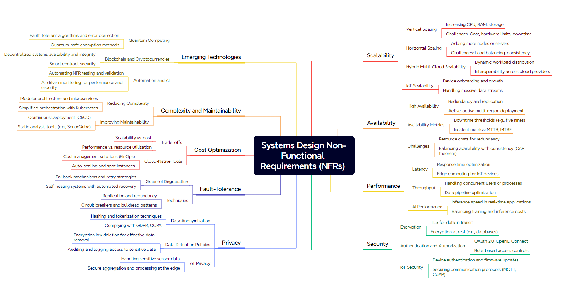
Making NFRs Measurable: The SRE Way with SLIs and SLOs

Having a list of NFRs like "availability" or "performance" is a good start, but it's still too vague for rigorous engineering. How do you measure "availability"? How fast is "performant"? At Google, this ambiguity is resolved through the discipline of Site Reliability Engineering (SRE), which provides a precise vocabulary for defining and measuring these attributes.

As explained in the video, we move from vague goals to concrete targets using this hierarchy:

1. Service Level Indicator (SLI): A direct, quantitative measure of some aspect of your service. This is what you measure. It should be a ratio of "good events" to "total valid events."

   • Availability SLI: (number of successful requests) / (total valid requests)
   • Latency SLI: (number of requests faster than threshold T) / (total valid requests)

2. Service Level Objective (SLO): A target value or range for an SLI over a time window. This is how good the service needs to be. It is an internal agreement that sets expectations for the engineering team.

   • Availability SLO: 99.9% of requests will succeed over a rolling 28-day window.
   • Latency SLO: 99% of requests will be served in under 200ms over a rolling 28-day window.

3. Error Budget: This is the most powerful concept here. It's simply 1 - SLO. If your availability SLO is 99.9%, your error budget is 0.1%. This budget represents the acceptable level of unreliability. It can be "spent" on risky feature launches, planned maintenance, or unavoidable outages. The error budget provides a data-driven framework for balancing reliability with the pace of innovation. If the budget is spent, all new feature launches are frozen until the service is back within its SLO.

4. Service Level Agreement (SLA): This is a business or legal contract with customers that defines the consequences of failing to meet certain objectives (often a subset of the SLOs). A broken SLA might result in financial penalties, while a broken SLO triggers an internal engineering response.

Defining SLOs for the most critical NFRs is the cornerstone of data-driven architectural analysis. It gives you a precise yardstick against which you can measure your different design alternatives.

Analyzing the Alternatives

With clear, measurable NFRs and SLOs defined, you can now systematically evaluate your architectural options. This process can happen in two phases: qualitative analysis to filter options, and quantitative analysis to make the final decision.

Phase 1: Qualitative Analysis

In the early stages, you may not have enough data for a full quantitative breakdown. A qualitative analysis allows you to do a "first pass" comparison based on the known properties of different architectural patterns.

The key idea here is to create a matrix comparing your architectural alternatives against your most important NFRs. Even if you only use a simple scoring system (e.g., --, -, +, ++), this exercise forces you to articulate why one option is better than another for a given characteristic.

For example, if comparing a microservices architecture to a modular monolith for a system where "time to market" (and thus deployability and testability) is paramount, the qualitative analysis would likely favor microservices, while acknowledging its trade-offs in operational complexity and cost. This structured comparison helps narrow the field to the most plausible candidates.

Phase 2: Quantitative Analysis with Back-of-the-Envelope Calculation

For the remaining viable alternatives, you need to go deeper. This is where you use back-of-the-envelope calculations to ground the trade-offs in concrete numbers. Your 15 years of experience as a programmer have given you an intuition for how systems behave; this is the process of formalizing and validating that intuition with numbers.

The goal is not to produce perfectly accurate forecasts, but to get within an order of magnitude. This is usually enough to reveal the true costs and benefits of each design.

Let's apply this framework. For each architectural alternative, you should estimate the key metrics tied to your SLOs.

The Estimation Framework:

1. Clarify the Goal: What are you estimating? (e.g., peak QPS, 1-year storage cost).
2. State Assumptions: Be explicit. (e.g., "Assuming 100M Daily Active Users, with 10% writing and 90% reading," "Assuming a 3x replication factor").
3. Decompose: Break the problem down. (e.g., To get storage cost, first find daily data ingress, then apply retention and replication, then apply cost per GB).
4. Estimate Components: Use simple math and round aggressively.
5. Combine and Sanity Check: Does the final number seem reasonable?

Let's see this in action with another video that provides a quick walkthrough.

Applying Quantitative Analysis to Make a Decision

Let's revisit the synchronous vs. asynchronous item availability architecture from the last lesson and apply this thinking.

• Business Goal: Provide item availability information on a product page.
• Availability SLO: 99.9% of requests succeed.
• Latency SLO: 95% of requests return in < 150ms.

Alternative A: Synchronous Aggregation

• Assumptions: 23 dependent service calls in a chain. To meet a 99.9% SLO, each service must have an availability of 0.999^(1/23) ≈ 99.995% (five nines).
• Quantitative Analysis:
  • Cost: Achieving five-nines reliability for 23 services is astronomically expensive in terms of infrastructure and operational overhead.
  • Latency: The p95 latency is the sum of the p95 latencies of all 23 calls. This makes the 150ms SLO nearly impossible to meet without heroic optimization on every single service.
  • Result: This architecture is quantitatively shown to be too expensive and too slow.

Alternative B: Asynchronous Materialized View

• Assumptions: The request path now involves only 2 services (e.g., API gateway, materialized view service). Data staleness is acceptable up to 30 seconds.
• Quantitative Analysis:
  • Cost: To meet the 99.9% SLO, the two user-facing services now need 0.999^(1/2) ≈ 99.95% availability—a much more achievable and cheaper target. The other 21 backend services can have much looser SLOs, further reducing cost.
  • Latency: The p95 latency is a single read from a local data store, easily meeting the 150ms SLO.
  • Trade-off (Quantified): The NFR for data freshness can be defined: p99 data staleness < 30 seconds. We can now design the asynchronous pipeline to meet this specific objective.
  • Result: This architecture is quantitatively superior on cost, latency, and availability, while making a specific, measurable trade-off on data freshness.

The numbers make the choice clear. By defining NFRs and quantifying them, you have moved from a vague preference to a defensible engineering decision.

Conclusion

In this lesson, we've built the analytical machinery required to evaluate complex architectural choices. Moving from vague goals to concrete metrics is the key to transforming architectural design from an art into an engineering discipline.

Here are your key takeaways:

• Translate Business to Engineering: Non-Functional Requirements (NFRs) are the technical embodiment of business goals. Your first job is to perform this translation.
• Measure What Matters with SLOs: Vague NFRs like "availability" become powerful decision-making tools when defined as precise Service Level Objectives (SLOs) based on measurable Service Level Indicators (SLIs). This is the standard at Google and a best practice industry-wide.
• Use a Phased Approach: Start with qualitative analysis to compare alternatives against NFRs and filter your options. Then, use quantitative analysis for the final decision.
• Ground Decisions in Numbers: Back-of-the-envelope calculations are your tool for quantitative analysis. By estimating traffic, storage, and other key metrics, you can make the costs and benefits of each trade-off explicit and tangible.

In our previous lesson, we learned to generate options. Now, we have a framework to evaluate them. In our next lesson, we will focus on synthesizing principles from canonical systems (e.g., Spanner, GFS, Dynamo) to design a novel solution for a given large-scale problem. We will start putting all these skills together—generating, evaluating, and synthesizing—to tackle complex design challenges from first principles.