Introduction
In our previous lesson, we built a formal vocabulary for classifying system failures, distinguishing between crash, omission, Byzantine, and gray failures. This framework allows us to precisely define a system's fault model. Now, we move from what can fail to how we detect that a failure has occurred.
This lesson focuses on the mechanisms for failure detection. We'll start by exploring the fundamental challenge: in an asynchronous distributed system, it's impossible to perfectly distinguish a crashed node from a merely slow or temporarily unreachable one. This uncertainty forces us to treat failure detection as a probabilistic exercise. We will analyze the most common approach, heartbeating, and its inherent trade-offs. We will then dive deep into a more sophisticated and flexible method used in many modern systems like Apache Cassandra: the Phi (φ) Accrual Failure Detector.
The Ambiguity of Timeouts
The first step in handling a fault is detecting it. The mechanism for this is called a failure detector. Ideally, we'd want a perfect detector that instantly and accurately tells us if a node has crashed. However, in the real world of asynchronous networks, this is not achievable.
To understand why, let's watch a brief segment from Martin Kleppmann's lecture series on distributed systems. He clearly explains why timeouts, the most common tool for detecting failures, are inherently ambiguous.
Distributed Systems 2.4: Fault tolerance
This video explains the fundamental problem with using timeouts for failure detection in partially synchronous or asynchronous systems.
Please watch the section from detecting a fault. As you watch, focus on the list of reasons why a timeout might occur. Note that a node crash is only one of several possibilities. This ambiguity is the central problem that failure detection mechanisms must navigate.
As Kleppmann explains, the absence of a message could be due to a node crash, network message loss (in either direction), network delay, or a long process pause (like garbage collection). A simple timeout cannot distinguish between these cases. This leads to a fundamental trade-off:
- Aggressive Timeout (short): Leads to fast detection of actual crashes but also a high number of false positives, where a healthy but slow node is incorrectly declared dead. This can cause unnecessary failovers and system instability.
- Conservative Timeout (long): Reduces false positives but increases the time it takes to detect a genuine crash (mean time to detection, or MTTD), potentially impacting availability.
This means we can't have a perfect failure detector. Instead, as the video also mentions, we aim for an eventually perfect failure detector—one that may be wrong temporarily but will eventually converge on the correct status of a node.
Heartbeats: The Standard Mechanism
The most common implementation of a failure detector is based on heartbeats. A heartbeat is a periodic message sent by a component to signal that it is alive and functioning. A monitor receives these messages and uses their presence—or absence—to infer the health of the sending component.
To formalize our understanding of this core mechanism, we will read through a blog post that provides an excellent overview.
Heartbeats in Distributed Systems
This article breaks down the components of a heartbeat system and the crucial trade-offs involved in configuring it.
Please read the first three sections of the article: Read the introduction and What are Heartbeat Messages for a basic definition. Continue through Core Components and Deciding Intervals. Pay close attention to the discussion of heartbeat interval and timeout threshold. This is the classic trade-off between detection speed and false positives we just discussed. Finally, read about the Push vs Pull models. Think about which model places more load on the monitored nodes versus the monitoring system.
The reading highlights that designing a heartbeat system isn't just about sending a message; it's about making deliberate design choices. The key parameters are:
- Heartbeat Interval: How often the "I am alive" message is sent.
- Timeout Threshold: How long the monitor waits without a heartbeat before declaring a node as failed. A common practice is to set this to a multiple (e.g., 3-5x) of the interval to tolerate transient network packet drops.
- Model:
- Push: The monitored node sends heartbeats to a monitor. This is common for service health checks.
- Pull: The monitor polls the node (e.g., "Are you there?"). This is common for infrastructure monitoring, like a load balancer checking its backends.
The core problem remains: a fixed timeout is a blunt instrument. It's a static, binary decision in a dynamic, analog world. A single timeout value that works well on a low-latency local network will perform poorly for a service operating across continents, where network jitter is much higher. This inflexibility is what motivates more advanced approaches.
Phi (φ) Accrual Failure Detectors
What if, instead of a binary "alive" or "dead" output, a failure detector could provide a level of suspicion? This would allow different applications to react differently based on their tolerance for risk. An application might take a low-risk precautionary measure at a low suspicion level, and only trigger a high-impact failover when the suspicion is very high.
This is the core idea behind accrual failure detectors, and the most famous implementation is the Phi (φ) Accrual Failure Detector, originally detailed in a 2004 paper and later popularized by its use in the Apache Cassandra database.
The Φ detector moves away from fixed timeouts and instead uses a statistical approach based on the history of heartbeat arrivals.
The φ Accrual Failure Detector
This is the original paper that introduced the ϕ accrual failure detector. We will focus on the motivation and the core mechanism.
Please focus on the following two key sections of the paper: Read Section I, "Introduction" (pages 1-2). The master/worker example provided here is an excellent illustration of why a continuous suspicion level is more powerful than a simple boolean output. It decouples the application's policy from the monitoring mechanism. Next, read Section IV, "Implementation of the φ Accrual Failure Detector" (pages 5-6). This is the heart of the mechanism. Your goal is to understand the definition of ϕ: \phi(t_{now}) = -\log_{10}(P_{later}(t_{now} - T_{last})) Break this down: t_{now} is the current time. T_{last} is the time the last heartbeat was received. P_{later}(t) is the probability that a heartbeat interval is longer than t. This is calculated by modeling the distribution of recent heartbeat inter-arrival times (stored in a sliding window) as a normal distribution.
Let's unpack the elegance of this formula. The value represents the probability of a heartbeat being this late, based on recent network behavior.
- If a heartbeat arrives on time, this probability is high (close to 1), and is low (close to 0).
- As a heartbeat becomes overdue, the probability of it being that late gets smaller and smaller, and the value grows.
The function maps this probability onto a more intuitive, roughly linear scale. A value of 1 means there's about a 10% chance that the heartbeat is simply late and not lost (i.e., we have a 10% chance of a false positive if we suspect now). A value of 2 corresponds to a 1% chance, 3 to 0.1%, and so on.
The diagram below illustrates this flow. Heartbeat arrival times are collected, used to estimate a probability distribution, which then allows for the calculation of .
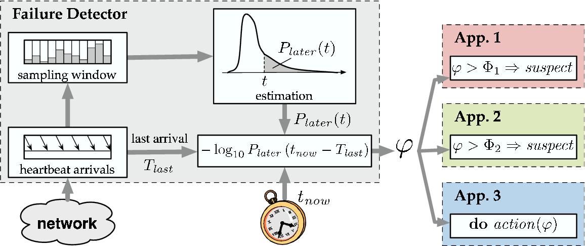
This approach is powerful because it is adaptive. It automatically adjusts to network conditions. During periods of high latency and jitter, the calculated distribution will be wider, and the detector will be more tolerant of late heartbeats. During stable periods, it will be tighter and more aggressive.

Conclusion
In this lesson, we explored the crucial task of failure detection. We established that due to the nature of asynchronous systems, perfect detection is impossible, forcing us to deal with probabilities and trade-offs.
Here are the key takeaways:
- The Detection Dilemma: Simple timeout-based heartbeats force a difficult choice between fast detection (with a high risk of false positives) and reliable detection (which is slow to react to real failures).
- Fixed vs. Adaptive: A fixed timeout is a static solution for a dynamic problem. It cannot adapt to changing network conditions, leading to poor performance in real-world environments with variable latency.
- Accrual Detectors: The accrual detector offers a more flexible abstraction by providing a continuous suspicion level rather than a binary output. It quantifies the probability that a node has failed based on a statistical model of its recent heartbeat arrivals.
- Decoupling Policy from Mechanism: By outputting a value, the detector allows applications to implement their own failure response policies (e.g., "reroute traffic at , declare dead at "). This decouples the what (application logic) from the how (failure monitoring).
The way a system handles failure detection has profound implications for its stability. An overly aggressive detector can trigger a "thundering herd" problem, where many clients simultaneously declare a healthy service dead and attempt to failover, creating a cascading failure. In our next lesson, we will investigate these cascading failures in depth, analyzing their common patterns and the mechanisms used to prevent them.