Hello! Welcome to your first lesson in the Game Balancing in Strategy Games course. I'm excited to get started and help you build a more formal, mathematical toolkit for your work as a game designer.
This first module is all about building a solid statistical foundation. Many of the complex balancing challenges in RTS and grand strategy games can be better understood and solved by looking at player data through a statistical lens.
In this lesson, we will focus on the most fundamental way to summarize data: measures of central tendency. You'll learn to interpret the mean, median, and mode to analyze common types of game data, like player wealth or match duration, which are often "skewed." Understanding this is the first step toward moving from intuition-based balancing to a more data-informed approach.
What are Mean, Median, and Mode?
Let's start with a quick definition of our three key terms. You are likely familiar with them, but a precise definition is always a good starting point.
- Mean: This is the most common type of "average." It's calculated by summing all the values in a dataset and dividing by the count of those values.
- Median: This is the middle value in a dataset that has been sorted in order. If there's an even number of values, the median is the average of the two middle values. Exactly 50% of the data is below the median.
- Mode: This is simply the value that appears most frequently in a dataset.
In a perfectly symmetrical dataset, like the outcomes of rolling a fair six-sided die many times, these three values would be very close to each other. However, game data is rarely so neat.
Why the "Average" Can Be Misleading: Skewed Data
In strategy games, many important metrics are not symmetrical. Consider the amount of gold a player has at the 10-minute mark in an RTS.
- Most players might have a modest amount, say between 2000-3000 gold.
- A few players who are doing exceptionally well ("snowballing") might have 8000 gold.
- A couple of players who were rushed and lost their expansion might have only 500 gold.
If you just calculated the mean (the average), the few players with huge amounts of gold would pull the average up, giving you a distorted picture of the typical player's economic state. This is called a skewed distribution.
To see this in action, let's watch a short video that uses a classic game example to illustrate this exact point.
Mean Vs Median. When to use which one.
This video from Six Sigma Academy Amsterdam uses player spending data in Street Fighter 2 to clearly explain why the mean can be misleading and how it differs from the median.
Please watch from the beginning until 02:24. Pay close attention to how the single extreme value of $5000 affects the mean, but has no real impact on the median.
As the video shows, the mean is sensitive to outliers—extreme values that lie far from the rest of the data. The median, on the other hand, is resistant to them. This is a critical distinction for game balance.
Visualizing and Interpreting Skew
We can describe the "shape" of a dataset by its skewness. The relationship between the mean, median, and mode gives us a clear signal about the direction of the skew.
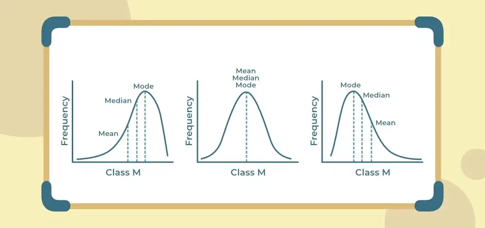
- Symmetrical Distribution (e.g., a Bell Curve): The data is evenly distributed around the center. Here, Mean ≈ Median ≈ Mode.
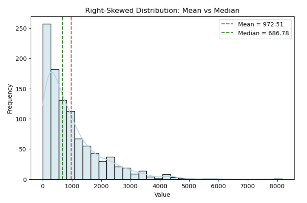
- Right-Skewed Distribution (Positively Skewed): The distribution has a long "tail" of high values to the right. This is very common for metrics like player wealth, kill counts, or time played. In this case, the outliers pull the mean to the right, so Mean > Median.
- Left-Skewed Distribution (Negatively Skewed): The distribution has a long tail of low values to the left. This is less common, but you might see it in data like "time remaining in a timed mission," where most players finish close to the deadline. Here, the outliers pull the mean to the left, so Mean < Median.
This next video provides a great visual walkthrough of these concepts.
Symmetric, right skewed (positively), and left skewed (negatively) distributions
This video from Dane McGuckian clearly illustrates how the mean, median, and mode behave in symmetric, right-skewed, and left-skewed distributions.
Watch from the beginning to 04:27. Focus on the core idea: the mean is always 'pulled' toward the long, skinny tail of the distribution.
Here is a concrete example of what a right-skewed distribution looks like with real data. Notice how the bulk of the data is on the left, and the mean is pulled to the right of the median by the long tail.
Test your understanding!
You are analyzing match duration data for a new RTS map. The data shows:
- Mean match duration: 25 minutes
- Median match duration: 18 minutes
- Mode match duration: 15 minutes
- What kind of distribution does this data likely have?
- What does this tell you about the matches being played on this map?
- If your design goal was for the "typical" game to last around 20 minutes, which measure gives you a more accurate picture of the typical player experience, and why?
Show answer
- The data is right-skewed, because the mean is significantly greater than the median (Mean > Median > Mode).
- This suggests that while most matches are relatively short (around 15-18 minutes), there is a subset of very long, drawn-out matches that are "pulling" the average duration up to 25 minutes. These could be late-game stalemates or other pacing issues that affect a minority of games.
- The median (18 minutes) gives a more accurate picture of the typical player experience. It tells us that 50% of games are finishing in 18 minutes or less. The mean is being distorted by the long-tail of unusually long games. If you based your balancing decisions on the mean, you might try to shorten the "average" game, when in fact the typical game is already shorter than your 20-minute target. The real issue to investigate might be what's causing those exceptionally long matches.
Application: Analyzing Real Game Data
Let's look at how these concepts are used in practice. The following article analyzes a dataset from a mobile game to understand player engagement and retention. You don't need to worry about the code, just focus on the author's interpretation of the statistics.
Analyzing Player Retention and Engagement Using Data ...
This article, 'Analyzing Player Retention and Engagement Using Data ...', provides a great case study of interpreting descriptive statistics from a real game.
Read the following parts of the article: The section after the first df.describe() command, starting with 'The max value for responses...' It shows how to spot skew just by comparing the mean and median. The section under 'Plot distributions for key metrics', focusing on the interpretation of the 'Distribution of Player Logins' histogram. The section where the author runs df['retention_days'].describe(), and the paragraph that follows it, starting with 'The mean retention period is 52.48 days...' The interpretation of the 'Distribution of Player Retention Period' histogram that follows.
Notice how the author repeatedly points out the large difference between the mean and the median for metrics like logins and retention days. They correctly interpret this right-skew not as a statistical error, but as a crucial insight: there's a small group of highly engaged, long-term players and a very large group of players who churn quickly. For a game designer, this immediately helps segment the player base and raises questions about the new player experience versus the elder game.
Beyond the Textbook: Choosing the Right Measure for the Right Decision
So far, the rule seems simple: "if the data is skewed, use the median." While this is good for understanding the typical case, it's not always the best for making decisions. Your goal as a designer is to make better decisions, and for that, the choice of metric should be driven by the decision you need to make.
This final article challenges the conventional wisdom and provides a more sophisticated framework that is directly applicable to your work.
Mean or median? Choose based on the decision, not ...
This article from Towards Data Science, 'Mean or median? Choose based on the decision, not the distribution', argues that your analytical goal should determine which measure you use.
Please read the introduction, the three examples under 'Decision analysis courses taught me a different approach...', and the 'Conclusions' section. Pay close attention to Example 3 ('A company considering an expansion').
The key insight here is powerful:
- Use the Median when your goal is to understand or communicate the typical experience and avoid distortion from outliers. For example: "What is the typical time-to-kill for a rifleman vs. a tank?"
- Use the Mean when your goal involves a total or aggregate. The article's salary example is perfect: to get the total cost, you must use the mean salary, not the median. In games, this applies to things like:
- Total Damage: The total damage a unit will do over its lifetime is its average damage per hit (mean) times its number of hits. A high-damage critical strike (an outlier) is a real event that contributes to the total and must be part of the mean calculation for accurate balancing.
- Total Revenue: For free-to-play games, total revenue is
mean revenue per player×number of players. The median revenue might be $0, but the mean, pulled up by high-spending "whales," is essential for business forecasting.
Key Takeaways and Next Steps
This lesson is a crucial first step. By understanding how to interpret measures of central tendency, you can extract much more meaningful insights from raw game data.
- Mean, median, and mode describe the center of your data, but they tell different stories.
- Game data is often right-skewed, with a long tail of high-value outliers (e.g., super-rich players, extremely long matches).
- In a skewed distribution, the mean is pulled toward the tail, while the median remains more stable. This difference is a signal of skew.
- Interpreting skew gives you insights into player behavior and helps you segment your audience (e.g., casuals vs. hardcore).
- The choice between mean and median should be driven by your analytical goal: use the median for the typical experience and the mean when you care about the total effect.
In our next lesson, we will build on this by looking at measures of spread. Now that we know how to find the center of our data, we need to ask: how consistent is it? We'll explore variance and standard deviation to quantify the spread and predictability of game outcomes, like the damage range of a weapon or the final score in a match.