Vector and Matrix Fundamentals

1. Vectors: The Building Blocks of Data

In machine learning and computer vision, we need a way to represent data numerically. Whether it's the features of an object, the color of a pixel, or the parameters of a model, we use vectors.

At its core, a vector is simply an ordered list of numbers. To get a formal definition and see how these are represented, let's start with our first reading.

As you've just read, while vectors can be abstract concepts, for our purposes, we'll primarily think of them as arrays of numbers. A vector in ${\mathbb{R}}^n$ is a list of $n$ real numbers, which we can use to represent a point in an $n$-dimensional space.

For example, in computer vision, a single color pixel is often represented by a vector of three numbers, like $[R,G,B]$, corresponding to the intensity of red, green, and blue. This is a vector in ${\mathbb{R}}^3$.

Key Vector Operations

From the reading, you've seen two fundamental operations. Let's formalize them.

1. Vector Addition

If we have two vectors $\mathbf{u}$ and $\mathbf{v}$ of the same dimension $n$, their sum $\mathbf{w}=\mathbf{u}+\mathbf{v}$ is found by adding the corresponding elements:

This operation is commutative ($\mathbf{u}+\mathbf{v}=\mathbf{v}+\mathbf{u}$) and associative ($(\mathbf{u}+\mathbf{v})+\mathbf{w}=\mathbf{u}+(\mathbf{v}+\mathbf{w})$).

2. Scalar Multiplication

Multiplying a vector $\mathbf{v}$ by a single number (a scalar) $\alpha$ scales the vector. Every element of the vector is multiplied by the scalar:

Geometrically, this changes the vector's magnitude (length) but not its direction (unless $\alpha$ is negative, in which case the direction is reversed).

This concludes the first part of our lesson. When you're ready, you can continue to the next section on matrices.

2. Matrices: Organizing Data in Grids

If a vector is a list of numbers, a matrix is a rectangular grid of numbers, arranged in rows and columns. This is an incredibly powerful structure. For instance, a grayscale image can be directly represented as a matrix where each entry is the brightness of a pixel.

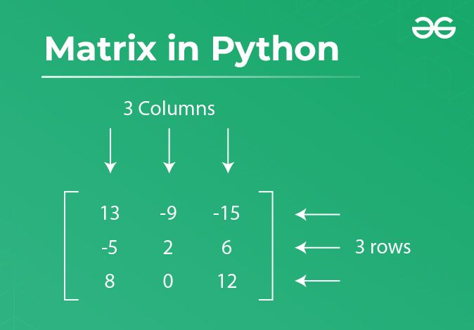
A matrix with $m$ rows and $n$ columns is said to have dimensions $m\times n$. We often denote it as $\mathbf{A}\in {\mathbb{R}}^{m\times n}$.

Let's return to our primary resource to explore matrices and their fundamental operations.

Key Matrix Operations

As you saw, the basic operations for matrices are direct extensions of what we learned for vectors.

1. Matrix Addition and Scalar Multiplication

Just like with vectors, matrix addition and scalar multiplication are performed element-wise.

• Addition: Two matrices $\mathbf{A}$ and $\mathbf{B}$ can be added only if they have the same dimensions. The resulting matrix $\mathbf{C}=\mathbf{A}+\mathbf{B}$ has entries $c_{ij}=a_{ij}+b_{ij}$.
• Scalar Multiplication: Multiplying a matrix $\mathbf{A}$ by a scalar $\alpha$ results in a matrix $\mathbf{B}$ where each element is $b_{ij}=\alpha \cdot a_{ij}$.

2. Matrix Transposition

The transpose of a matrix $\mathbf{A}$, denoted ${\mathbf{A}}^T$, is a new matrix where the rows of $\mathbf{A}$ become the columns of ${\mathbf{A}}^T$, and vice versa. If $\mathbf{A}$ is an $m\times n$ matrix, then ${\mathbf{A}}^T$ is an $n\times m$ matrix.

The entry in the $i$-th row and $j$-th column of ${\mathbf{A}}^T$ is the same as the entry in the $j$-th row and $i$-th column of $\mathbf{A}$. That is, $({\mathbf{A}}^T{)}_{ij}=A_{ji}$.

For example:
$\mathbf{A}=\left[\begin{array}{ccc}1& 2& 3\\ 4& 5& 6\end{array}\right]⟹{\mathbf{A}}^T=\left[\begin{array}{cc}1& 4\\ 2& 5\\ 3& 6\end{array}\right]$

Implementation in Python with NumPy

Since you have a background in Python, it's time to introduce the primary tool for numerical computing: NumPy. You have no prior experience with it, so let's start slowly. NumPy's main object is the ndarray (n-dimensional array), which we'll use to represent both vectors and matrices.

Here's how you'd perform the operations we've discussed.

import numpy as np

# Create a 2x3 matrix (2 rows, 3 columns)
A = np.array([[1, 2, 3], 
              [4, 5, 6]])

# Create another 2x3 matrix
B = np.array([[7, 8, 9],
              [10, 11, 12]])

# 1. Addition
C = A + B
print("A + B =\n", C)

# 2. Scalar Multiplication
D = 2 * A
print("\n2 * A =\n", D)

# 3. Transposition
A_T = A.T  # or A.transpose()
print("\nTranspose of A =\n", A_T)
print("\nShape of A:", A.shape)       # Will be (2, 3)
print("Shape of A_T:", A_T.shape) # Will be (3, 2)

Feel free to run this code on your own machine to get a feel for it. Make sure you have NumPy installed (pip install numpy).

Conclusion

Excellent work on completing your first lesson! You've taken the first crucial step into the mathematical world of computer vision.

Let's summarize the key takeaways:

• Vectors are ordered lists of numbers, representing points or directions in space.
• Matrices are rectangular grids of numbers, which can represent datasets, images, or transformations.
• Addition and scalar multiplication are element-wise operations for both vectors and matrices.
• Transposition is a fundamental matrix operation that swaps rows and columns, turning an $m\times n$ matrix into an $n\times m$ matrix.

These operations may seem simple, but they are the atomic units of the more complex algorithms you will build later.

Preview of the Next Lesson:
In our next lesson, we will move on to two of the most important operations in all of linear algebra: the dot product of vectors and matrix multiplication. You'll discover that matrix multiplication is not an element-wise operation, and understanding how it works is key to unlocking powerful techniques in machine learning.