Calculating Discrete Entropy

1. From Surprisal to Average Surprisal: Defining Entropy

In the last lesson, we found the "surprisal" of a single event. But how much information, on average, do we get from a system that produces many different events? For instance, a biased coin that lands on heads 90% of the time is quite predictable. On average, we won't be very surprised by its outcome. A fair coin, with a 50/50 split, is less predictable. On average, its outcomes are more surprising. Entropy is the measure of this average surprise.

To calculate an average, we take each outcome's value (its surprisal) and weight it by how often it occurs (its probability). We then sum these weighted values.

The following video from the StatQuest channel provides an excellent, intuitive derivation of entropy starting from this very idea of "average surprise."

As the video demonstrates, if a random variable $X$ can take on values $x_1,x_2,\dots ,x_n$ with probabilities $p(x_1),p(x_2),\dots ,p(x_n)$, the entropy $H(X)$ is the expected value of the surprisal:

This is conventionally written as:

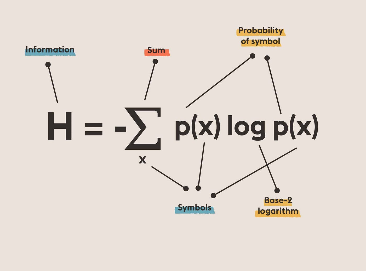
This formula is the heart of today's lesson. It gives us a single number that captures the total uncertainty of a probability distribution.

2. A More Formal View

While the "average surprisal" intuition is powerful, Shannon's definition of entropy can also be motivated from a more axiomatic, mathematical perspective, which aligns with your interests in formalism. One can start by listing desirable properties for a measure of surprise and find that only a logarithmic function will do. Entropy then emerges as the expected value of this function.

The following lecture from the University of Oxford formalizes this approach.

The lecturer also makes two important technical points:

• The base of the logarithm is a choice of units. In information theory, we almost always use base 2, and the unit is the bit. An entropy of 2.5 bits means that, on average, we need 2.5 binary questions (yes/no) to determine the outcome of an event drawn from that distribution.
• If a probability $p(x_i)$ is 0, we define $0{\log }_{2}0=0$. This makes sense intuitively: an impossible event contributes nothing to the overall uncertainty of the system.

3. Calculating Entropy: A Walkthrough

Now let's put the formula into practice. The calculation itself is straightforward once you have the probability distribution. We will work through a simple example step-by-step.

The following article provides a clear, practical guide to this calculation.

Let's re-trace the calculation from the article to ensure every step is clear.
We have a distribution with four outcomes (A, B, C, D) with the following probabilities:

• P(A) = 0.5
• P(B) = 0.25
• P(C) = 0.125
• P(D) = 0.125

The entropy is $H(P)=-\sum p(x){\log }_{2}p(x)$.

1. Term for A: $-(0.5\times {\log }_2(0.5))=-(0.5\times -1)=0.5$

2. Term for B: $-(0.25\times {\log }_2(0.25))=-(0.25\times -2)=0.5$

3. Term for C: $-(0.125\times {\log }_2(0.125))=-(0.125\times -3)=0.375$

4. Term for D: $-(0.125\times {\log }_2(0.125))=-(0.125\times -3)=0.375$

5. Sum the terms: $H(P)=0.5+0.5+0.375+0.375=1.75$ bits.

The result, 1.75 bits, is the average amount of information we gain upon learning the outcome from this source. It is also the theoretical lower limit for the average number of bits per symbol needed to encode messages from this source.

4. Interpreting the Result

The numerical value of entropy is directly related to the shape of the probability distribution.

• Low Entropy: A distribution with one very likely outcome and many unlikely ones is highly predictable. It has low uncertainty and therefore low entropy.
• High Entropy: A uniform distribution, where all outcomes are equally likely, is the most unpredictable. It has the highest possible uncertainty and therefore the maximum entropy for that number of outcomes.

This principle is fundamental to cybernetics. A system with high entropy (like a chaotic market) is inherently harder to predict and control than a system with low entropy (like a tightly regulated production line). Stafford Beer's work, which inspired you, is deeply concerned with how organizations can manage the high-entropy complexity of their environments.

Conclusion

In this lesson, we have moved from the information of a single event to the average information of an entire probability distribution. This measure, entropy, is a cornerstone of cybernetics and information theory.

Here are the key takeaways:

• Entropy measures average uncertainty. It is the expected value of the "surprisal" across all possible outcomes of a random variable.
• The formula is $H(X)=-\sum p(x){\log }_{2}p(x)$. The calculation involves summing the weighted surprisal of each outcome.
• The unit of entropy is the bit (when using log base 2), representing the average number of yes/no questions needed to identify an outcome.
• Entropy reflects the shape of a distribution. Uniform distributions have maximum entropy (high uncertainty), while peaked distributions have low entropy (high predictability).

You are now able to quantify the uncertainty of any simple discrete system, a crucial first step in analyzing information flows. In our next lesson, we will place this concept within its original context by describing Shannon's full model of a communication system, which includes a source, transmitter, channel, receiver, and destination. This will show how entropy dictates the fundamental limits of communication.