Hello! Welcome back to our course.
In our last lesson, we introduced the main players in any replacement decision: the defender (the asset you currently own) and the challenger (the best available replacement). We established that the decision to replace an asset is driven by economics, balancing the high initial cost of a new asset against the rising operating costs of an old one.
This brings us to a crucial question: What is the ideal amount of time to keep an asset? If we replace it too soon, we waste money by not getting the full value from our initial investment. If we keep it too long, we end up paying excessive amounts in maintenance and suffering from lower performance.
Today, we will learn how to find this economic "sweet spot." Our goal is to calculate the economic service life (ESL) for an asset by minimizing its equivalent annual cost. The ESL is a fundamental concept that tells us the optimal lifespan to use for an asset when comparing it to alternatives.
The Two Competing Costs
At the heart of the Economic Service Life calculation is a trade-off between two opposing cost trends:
-
Capital Costs (or Ownership Costs): This is the cost of acquiring and holding the asset. It's primarily the initial purchase price (
P) minus the asset's salvage or market value (S) at the time of disposal. When we spread this net cost over the asset's life, the annual share gets smaller the longer we keep it. Think of it as the "mortgage payment" on the asset; a longer term means lower annual payments. -
Operating Costs: These are the day-to-day costs of running the asset—maintenance, repairs, electricity, operator labor, etc. For most assets, especially mechanical or electronic ones like servers, these costs tend to increase over time as the asset wears out and becomes less efficient.
The Economic Service Life is the point where the sum of these two costs is at its lowest.
To understand this balancing act, please review the following resource. It introduces the concept and includes a helpful graph.
Economics for Engineers: Notes
This document from 'Economics for Engineers: Notes' explains the components of an asset's total annual cost and illustrates how they interact to create a minimum cost point.
Please read the section titled 'Economic Service Life' (pages 16-17). Pay close attention to the definitions of Capital Recovery Cost (CR(i)) and Operating Costs (OC(i)), and study the graph that shows how these two curves combine to form the Annual Equivalent Cost (AEC(i)) curve. Note the minimum point labeled n*.
As you saw in the reading, the total annual cost, which we'll call the Equivalent Uniform Annual Cost (EUAC), first decreases as the high initial capital cost is spread over more years. Eventually, however, the rising annual operating costs begin to dominate, causing the total EUAC to rise again. The lowest point on this U-shaped curve corresponds to the Economic Service Life (ESL).

Calculating the Economic Service Life
Now that we understand the concept, let's walk through the calculation. The process is straightforward but requires careful, year-by-year calculation:
- Gather your data for each potential year (
k) you might own the asset:- The initial cost,
P. For a new asset (a challenger), this is its purchase price. For an existing asset (a defender), this is its current market value. - The estimated salvage/market value at the end of each year,
S_k. - The estimated annual operating cost for each year,
AOC_k.
- The initial cost,
- For each possible life
k= 1, 2, 3, ... N years, calculate the total EUAC. - The ESL is the year
kthat has the minimum EUAC.
The general formula for the EUAC for a life of k years is:
EUAC_k = Capital Recovery + AW of Operating Costs
Where:
- Capital Recovery =
- AW of Operating Costs =
This looks complex, but it's just converting all costs incurred up to year k into an equivalent uniform annual series. Let's make this concrete with an example.
Replacement and Retention Decisions
This lecture presentation from Middle East Technical University provides a clear, worked-out example of an ESL calculation. We will adapt this example to walk through the steps.
Please review slides 7, 8, and 9, which present 'In Class Work 18.' Focus on the initial data provided in the table on slide 7 and observe how the 'Total AWn' is calculated for each year on slides 8 and 9. Note that the resource calculates 'Annual Worth of Cost,' which results in negative values. We will calculate the 'Annual Cost,' which is the positive equivalent.
Example Walkthrough
Let's use the data from the resource you just reviewed. An existing asset (a defender) has a current market value of $13,000. The interest rate is 10%. The estimated future market values and operating costs are:
| Year (j) | Market Value (MV) at end of year | Annual Operating Cost (AOC) for year j |
|---|---|---|
| 1 | $9,000 | $2,500 |
| 2 | $8,000 | $2,700 |
| 3 | $6,000 | $3,000 |
| 4 | $2,000 | $3,500 |
| 5 | $0 | $4,500 |
We need to calculate the EUAC if we keep the asset for 1 year, 2 years, 3 years, and so on.
Calculation for k = 1 year:
- Capital Recovery:
- and
- AW of Operating Costs: Only AOC for year 1 is relevant.
- . (Or simply, the AOC for the first year is $2,500).
- Total EUAC for k=1:
Calculation for k = 2 years:
- Capital Recovery:
- and
- AW of Operating Costs: We need the annual worth of both AOC_1 and AOC_2.
- Total EUAC for k=2:
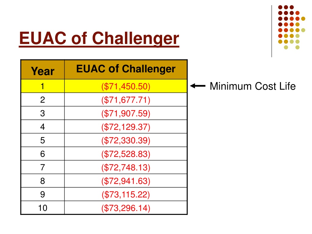
If we continue this process, we get the following table:
| Life (k) | Capital Recovery | AW of Operating Costs | Total EUAC |
|---|---|---|---|
| 1 Year | $5,300 | $2,500 | $7,800 |
| 2 Years | $3,681 | $2,595 | $6,276 |
| 3 Years | $3,415 | $2,717 | $6,132 |
| 4 Years | $3,670 | $2,886 | $6,556 |
| 5 Years | $3,429 | $3,150 | $6,579 |
The minimum total EUAC is $6,132, which occurs at k = 3 years.
Therefore, the Economic Service Life (ESL) of this asset is 3 years.
This is the number we would use as the "life" of the defender when comparing it to a challenger.
Test your understanding!
You are analyzing a new software server (a challenger) with an initial cost of $50,000. Your company's MARR is 12%. You have the following estimates:
| Year (k) | Market Value (MV) at end of year | Annual Operating Cost (AOC) for year k |
|---|---|---|
| 1 | $30,000 | $5,000 |
| 2 | $20,000 | $8,000 |
To find the EUAC for a service life of 2 years, which values would you use for P, S_k, AOC_1, and AOC_2 in your formulas?
Show answer
- P (Initial Cost): $50,000
- S_k (Salvage Value at k=2): $20,000
- AOC_1 (Operating Cost in Year 1): $5,000
- AOC_2 (Operating Cost in Year 2): $8,000
To complete the calculation, you would find the present worth of the two AOCs, convert that to an annual worth over 2 years, and add it to the capital recovery calculated using P=$50,000 and S_2=$20,000.
Conclusion
Today we've mastered a critical skill in replacement analysis: determining an asset's Economic Service Life. This isn't just an abstract calculation; it provides the most economically sound lifespan to use when evaluating an asset. Making decisions based on an asset's physical life or an arbitrary accounting period can lead to poor financial outcomes. The ESL gives us a data-driven basis for comparison.
- Key Takeaways:
- The Economic Service Life (ESL) is the service life in years that minimizes an asset's Total Equivalent Uniform Annual Cost (EUAC).
- This minimum cost is found by balancing two competing factors: the decreasing annual capital cost and the increasing annual operating cost.
- The calculation involves computing the total EUAC for each potential service life (1 year, 2 years, etc.) and selecting the year with the lowest value.
Preview of the Next Lesson
Now that we know how to calculate the ESL for a single asset, we are ready to perform a full replacement analysis. In our next lesson, we will determine the optimal replacement time for deteriorating assets. We will calculate the ESL for both the defender and the challenger and use those minimum annual costs to decide if we should replace the asset now, or wait.