Big-O Space Complexity: Memory Allocation Analysis

1. What is Space Complexity?

Just as time complexity describes how runtime scales with input size, space complexity describes how an algorithm's memory usage scales with input size.

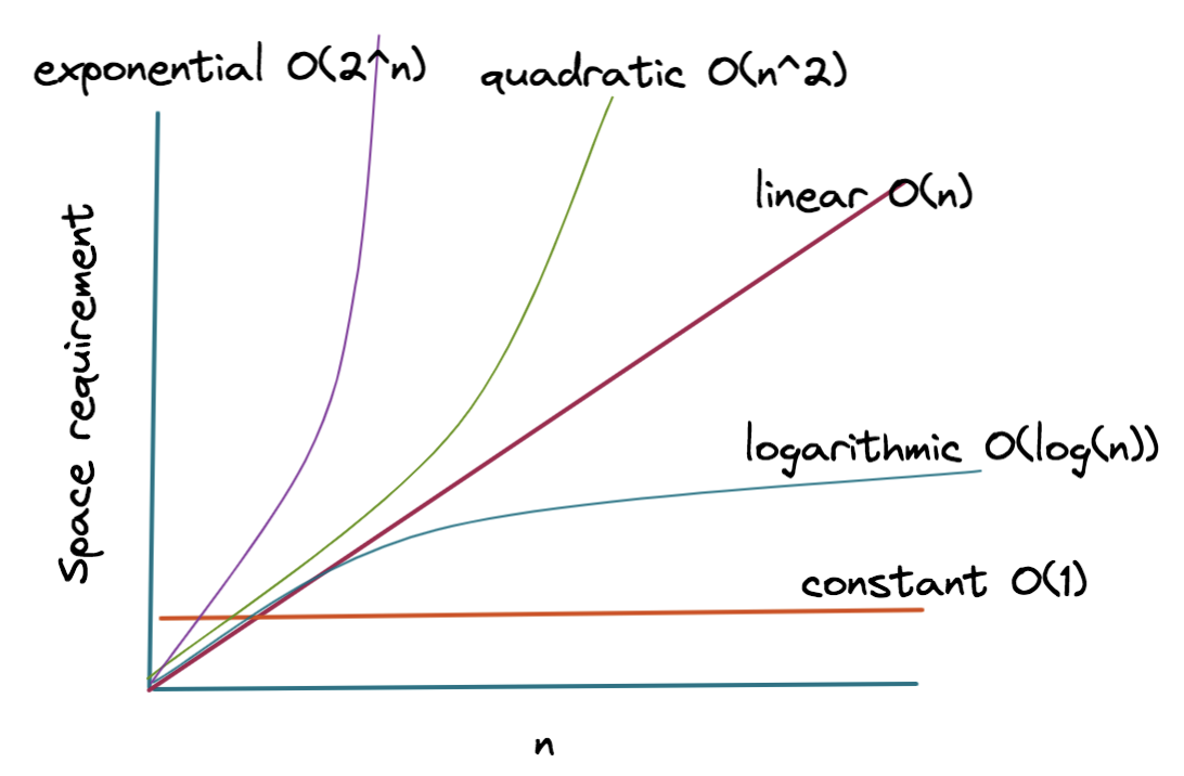
A crucial distinction in space complexity analysis is between total space and auxiliary space.

• Total Space Complexity: The total memory consumed by the algorithm, including the space taken up by the input data itself.
• Auxiliary Space Complexity: The extra or temporary space used by the algorithm, not including the space taken by the input.

In coding interviews, when an interviewer asks for the "space complexity," they are almost always referring to the auxiliary space complexity. This is because we want to measure the memory cost of the algorithm itself, independent of the storage cost of the data it operates on.

The following video provides a clear introduction to this concept.

2. A Quick Refresher: Stack vs. Heap Memory

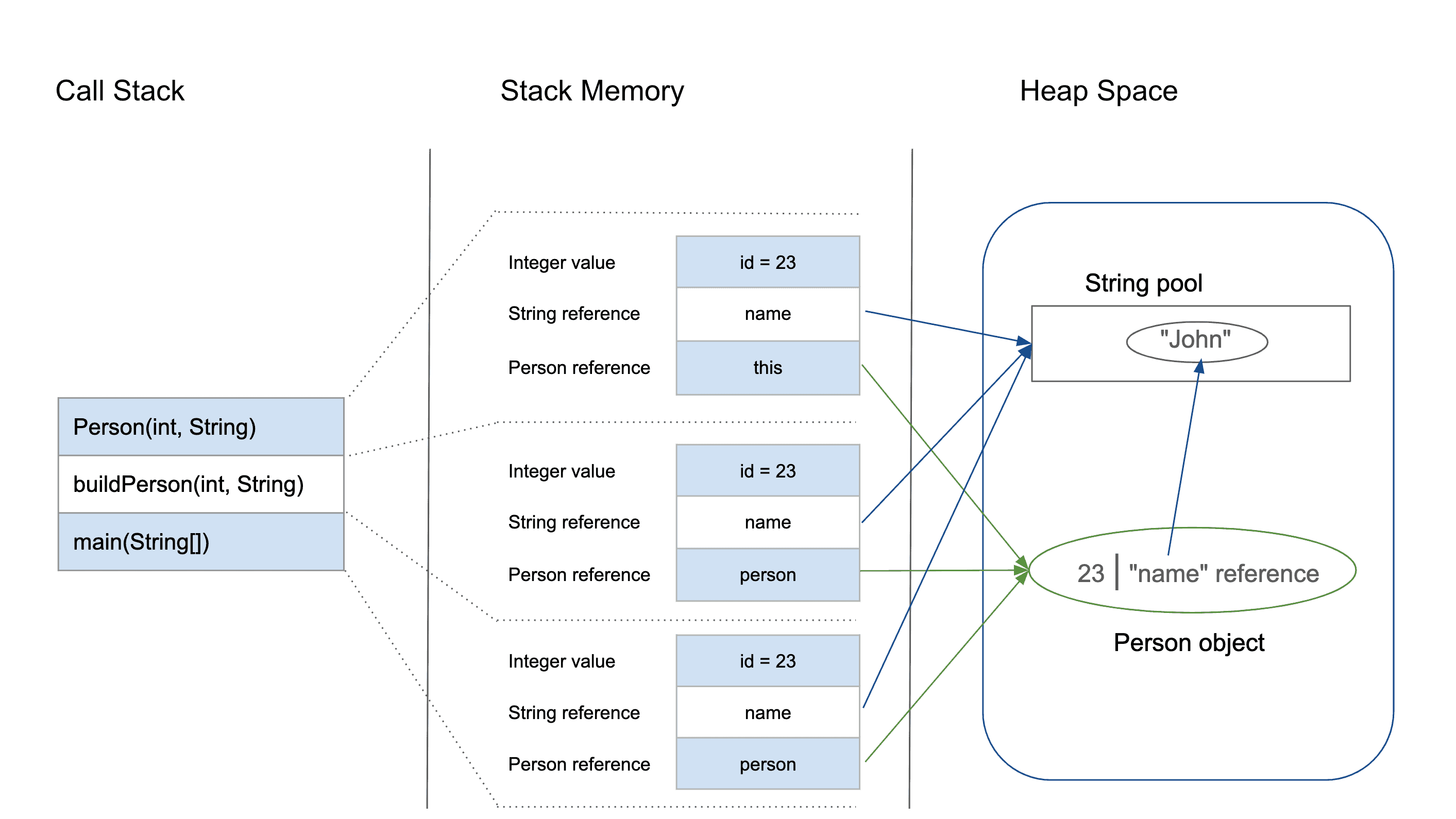
Since you work extensively with Java, you're already familiar with the concepts of Stack and Heap memory. This model is fundamental to understanding where space allocations occur.

• Stack Memory: Used for static memory allocation. It stores primitive local variables (like int, char, boolean) and references to objects. Crucially, it also manages function call frames. Each time a function is called, a new frame containing its local variables is pushed onto the call stack. This is the primary source of space usage in recursive algorithms.
• Heap Memory: Used for dynamic memory allocation. All objects created with the new keyword in Java, as well as complex data structures like arrays, lists, and maps that are created at runtime, are stored here. This is the primary source of space usage when you create new data structures within your algorithm.

3. Analyzing Space Complexity: Iterative Algorithms

Let's apply these ideas to iterative code. The space complexity is determined by the variables and data structures you allocate.

Constant Space Complexity: O(1)

An algorithm has O(1) auxiliary space complexity if the amount of extra memory it uses does not change with the input size. It uses a fixed number of variables.

A classic example is a linear search in an array.

boolean linearSearch(int[] array, int target) {
    for (int i = 0; i < array.length; i++) { // 'i' is O(1) space
        if (array[i] == target) {
            return true;
        }
    }
    return false;
}

Even though the input array takes O(N) space, the linearSearch algorithm itself only uses a few variables (i, target, and the reference to array). The number of these variables is constant regardless of whether the array has 10 elements or 10 million. Therefore, its auxiliary space complexity is O(1).

The following video explains this using the linear search example.

Linear Space Complexity: O(N)

An algorithm has O(N) auxiliary space complexity if the extra memory it uses grows linearly with the input size N. This typically happens when you create a new data structure whose size depends on the input.

Consider a function that creates a copy of an array:

int[] copyArray(int[] array) {
    int n = array.length;
    int[] newArray = new int[n]; // Allocates O(N) space on the heap

    for (int i = 0; i < n; i++) {
        newArray[i] = array[i];
    }
    return newArray;
}

Here, the line new int[n] allocates a new block of memory on the heap whose size is directly proportional to the input array's length. Thus, the auxiliary space is O(N).

Sometimes, O(N) space usage can be less obvious, especially with language features like string immutability in Java.

import java.util.ArrayList;
import java.util.List;

class Solution {
    public List<Integer> getEvenNumbers(int[] nums) {
        List<Integer> evens = new ArrayList<>(); // A dynamic array
        for (int num : nums) {
            if (num % 2 == 0) {
                evens.add(num);
            }
        }
        return evens;
    }
}

4. Analyzing Space Complexity: Recursive Algorithms

For recursive algorithms, the primary source of auxiliary space complexity is the call stack. Each recursive call adds a new frame to the stack, and the maximum depth of this stack during execution determines the space complexity.

Linear Space: O(N)

If a function calls itself N times before reaching a base case, the stack depth will be N.

A classic example is the factorial function fact(n). The call chain is fact(n) -> fact(n-1) -> ... -> fact(1), creating n frames on the call stack.

A more interesting example is the naive recursive Fibonacci algorithm. Although it has an exponential O(2^N) time complexity due to recomputing values, its space complexity is only O(N). Why? Because the recursive calls are executed sequentially. The call stack only needs to go down one path at a time. The maximum depth of the call stack will be N.

Logarithmic Space: O(log N)

Algorithms that follow a divide-and-conquer approach, where the problem size is halved at each step (like binary search), often have a logarithmic space complexity for their recursive implementation. The number of nested calls (stack depth) is proportional to log N.

However, be careful! Other memory allocations can dominate the stack space. The video below discusses Quicksort and Merge Sort, which are great examples.

This trade-off is a perfect example of the kind of analysis expected from a Principal Engineer. Merge Sort guarantees O(N log N) time but requires O(N) space. Quicksort has a better average-case space complexity of O(log N) but its time complexity can degrade to O(N²).

Conclusion

You can now analyze both the time and space complexity of iterative and recursive algorithms. This provides a complete picture of an algorithm's performance profile.

Key Takeaways:

• Auxiliary Space is Key: In interviews, "space complexity" almost always means the extra space used by your algorithm, not including the inputs.
• O(1) Space: Your algorithm uses a fixed amount of memory, regardless of input size. This is typical for simple loops with a few variables.
• O(N) Space: Your algorithm's memory usage scales linearly with the input size. This usually involves creating a new data structure (e.g., array, list, hash map) whose size depends on N.
• Recursion & The Call Stack: For recursive algorithms, space complexity is determined by the maximum depth of the call stack. This leads to O(N) for linear recursion (like factorial) and O(log N) for divide-and-conquer recursion (like binary search).
• Look for the Dominant Term: Always consider all sources of memory (stack and heap) and identify the one that grows the fastest. For Merge Sort, the O(N) heap allocation for the temporary array dominates the O(log N) stack space.

Next Lesson Preview:
We've now covered how to analyze the complexity of iterative algorithms and the space complexity of recursive ones. The final piece of this module is analyzing the time complexity of recursive algorithms. In the next lesson, we will introduce a powerful tool for this: recurrence relations and the Master Theorem.