From Constraints to Complexity: Navigating Problem Bounds

Hello! Welcome to the first lesson of our course. As a Senior Architect, you're accustomed to thinking about performance, scalability, and trade-offs at the system level. This module will sharpen that same intuition but apply it at the micro-level of individual algorithms—a crucial skill for coding interviews.

Today's goal is to master the very first step you should take when faced with any coding problem: translating the problem's constraints (like input size and time limits) into a "performance budget" for your algorithm. This will allow you to immediately rule out inefficient approaches and strategically target the right type of solution before you even start coding.

1. The "Why": Performance Budgeting in Coding Interviews

In your work, you perform back-of-the-envelope calculations for storage or QPS to guide system design. In a coding interview, you'll do something similar for algorithms. Problems on platforms like LeetCode or HackerRank don't run on infinitely fast machines; they execute your code within a containerized environment with a strict time limit, usually 1-2 seconds.

This time limit, combined with the processing power of the judge's server, creates an implicit limit on the total number of computational operations your code can perform. A widely accepted rule of thumb is that a typical online judge can execute roughly 100 million (10⁸) operations per second.

To understand the mechanics behind this, the following video provides a concise overview of how coding platforms evaluate your submissions. This "first principles" look at the infrastructure will help ground the rules we'll establish next.

LeetCode Feels Easy After This Reverse Runtime Trick

This video, 'LeetCode Feels Easy After This Reverse Runtime Trick' from AlgoMonster, explains the infrastructure behind online judges and why time limits matter.

Please watch the section from 01:02 to 02:41. It gives a glimpse into the backend process of code submission, execution in Docker containers, and the concept of a timeout. This context is key to understanding why we need to care about complexity.

By understanding that there's a finite operation budget, you can see that the choice of algorithm isn't just about correctness—it's about feasibility.

2. Mapping Input Size to Required Time Complexity

Now for the core skill of this lesson: using the input constraints to deduce the required time complexity. If your algorithm performs significantly more than ~10⁸ operations, it will result in a "Time Limit Exceeded" (TLE) error.

Let's say the input size is given by a variable N.

If N = 100,000 and your algorithm has a time complexity of $O (N^{2})$ , the number of operations will be roughly $(1 0^{5})^{2} = 1 0^{10}$ . This is far too high for a 1-second time limit.
If, for the same N, your algorithm is $O (N lo g N)$ , the operations would be around $1 0^{5} \times lo g_{2} (1 0^{5}) \approx 1 0^{5} \times 17$ , which is about 1.7 million operations. This is well within our budget.

This "reverse engineering" from constraints to complexity is one of the most powerful heuristics in a timed coding setting.

The following resources provide excellent, practical tables that you should aim to internalize. They are your cheat sheet for this process.

Knowing the complexity in competitive programming

The article 'Knowing the complexity in competitive programming' from GeeksforGeeks offers a clear, actionable table for this mapping.

Please read the section titled 'How to Determine the solution of a problem by looking at its constraints?'. Focus on the table that maps 'Constraints' (the value of n) to 'Worst time complexity'. This is the central piece of information for this lesson.

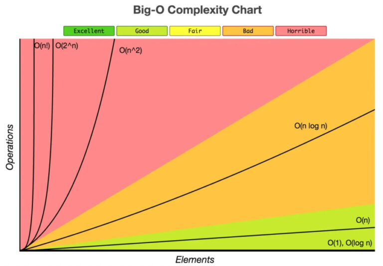
To give you a visual anchor for these numbers, here is a helpful summary chart.

Input Size to Complexity Mapping Table — This table provides a quick reference for mapping input size `n` to the required time complexity for your solution to be accepted within typical time limits.

Here is a summary of the most common and important mappings to commit to memory:

Input Size `N`	Required Time Complexity	Common Algorithm Types
`N` ≤ 20	$O (2^{N})$ , $O (N!)$	Brute-force recursion, backtracking (subsets, permutations)
`N` ≤ 500	$O (N^{3})$	Three nested loops, some dynamic programming
`N` ≤ 5,000	$O (N^{2})$	Two nested loops, basic graph traversals on dense graphs
`N` ≤ 100,000	$O (N lo g N)$	Efficient sorting, divide and conquer, heap algorithms
`N` ≤ 1,000,000	$O (N)$	Linear scan, two pointers, sliding window, hashing
`N` is very large	$O (lo g N)$ , $O (1)$	Binary search, direct mathematical formulas

This chart visualizes why this matters. As N grows, the operational cost of inefficient algorithms explodes.

Big-O Complexity Chart — This chart illustrates the growth rates of common time complexities. Notice how quickly the 'Bad' (Orange) and 'Horrible' (Red) complexities like $O(N^2)$ and $O(2^N)$ become infeasible as the number of elements increases.

Test your understanding!

You are given a coding problem with the following constraints for the input array nums: 1 <= nums.length <= 5 * 10^4. The time limit is 1 second.

Which of the following algorithmic complexities would you aim for?

$O (N^{2})$
$O (N)$
$O (N lo g N)$
$O (2^{N})$

Show answer

The correct answers are 2 ( $O (N)$ ) and 3 ( $O (N lo g N)$ ).

With N up to 50,000, an $O (N^{2})$ solution would perform roughly $(5 \times 1 0^{4})^{2} = 25 \times 1 0^{8} = 2.5 \times 1 0^{9}$ operations, which is too slow. An $O (2^{N})$ solution is only feasible for very small N (around 20-25).

An $O (N lo g N)$ solution would be approximately $5 \times 1 0^{4} \times lo g_{2} (5 \times 1 0^{4}) \approx 50, 000 \times 16 \approx 800, 000$ operations. An $O (N)$ solution would be around 50,000 operations. Both are safely within the ~10⁸ operation budget.

3. A Practical Example: Maximum Subarray Sum

Let's see how this works with a classic problem: finding the contiguous subarray with the largest sum. We won't implement the code now, but let's analyze the approaches.

Knowing the complexity in competitive programming

This section of the GeeksforGeeks article demonstrates three different algorithms for the same problem and analyzes their performance.

Read the part of the article that discusses the 'Maximum subarray sum' problem. Pay attention to the three methods described (O(n³), O(n²), and O(n)) and the final table showing their execution times for different values of n. This powerfully illustrates the real-world impact of choosing the right complexity.

As you saw, the $O (N^{3})$ and $O (N^{2})$ solutions are simple to conceptualize but quickly become impractical. If an interviewer presented this problem with an input size of N = 10^5, you would know immediately that a solution with nested loops iterating through all subarrays ( $O (N^{2})$ ) is not what they are looking for. This allows you to discard that idea and focus on finding the linear-time, $O (N)$ solution (Kadane's Algorithm), which we will cover later in the course.

4. A Note on Multiple Test Cases

Some competitive programming platforms present problems with multiple test cases within a single run. You might see constraints like:

1 <= T <= 1000 (where T is the number of test cases)
1 <= N <= 10^5
"The sum of N over all test cases does not exceed 10^6."

Don't be fooled by the T * N product, which could be as large as 1000 * 10^5 = 10^8. The crucial constraint is the last one. It tells you the total number of elements your algorithm will process across all test cases is at most 10^6. Therefore, an $O (N)$ algorithm for each test case will result in a total of $O (\sum N)$ operations, which is perfectly acceptable.

This final reading provides another perspective on the general principles we've discussed.

A Time Complexity Guide

This Codeforces blog post, 'A Time Complexity Guide', is written from a competitive programming perspective but its core principles are universal.

Please read the two untitled sections following the 'Big O Notation' section. The first part reinforces the '10⁷ - 10⁸ operations' rule. The second part explains the 'Sum of N over all test cases' constraint we just discussed. This will solidify your understanding of these nuances.

Conclusion

In this lesson, we established the foundational skill of performance estimation. You now have a framework for using a problem's constraints to define your algorithmic target before you begin designing a solution.

Key Takeaways:

The Performance Budget: Most online judges allow for ~10⁸ operations per second.
Constraints Guide Strategy: The input size N is the most important clue to the required time complexity.
Internalize the Mappings: Knowing that N=10^5 implies an $O (N lo g N)$ or $O (N)$ solution will save you critical time and guide your thinking.
Look Beyond a Single N: Be aware of how constraints can be specified across multiple test cases.

Next Lesson Preview:
Now that you can determine the target complexity for a given problem, the next step is to learn how to analyze the code you write to determine its complexity. In our next lesson, we will start with the basics: deriving Big-O time complexity for iterative algorithms by analyzing loop structures.

Recommended resources

1. The "Why": Performance Budgeting in Coding Interviews

2. Mapping Input Size to Required Time Complexity

3. A Practical Example: Maximum Subarray Sum

4. A Note on Multiple Test Cases

Conclusion