Softmax: From Logits to Probabilities

Introduction

In our last lesson, we established the critical role of non-linear activation functions like ReLU. We saw that they give our network the flexibility to learn complex patterns by transforming the outputs of each linear layer.

This leaves us with a network that can process an image and produce a set of raw numerical outputs from its final layer. We call these outputs logits. However, these logits aren't easily interpretable; they can be any number, positive or negative, and they don't give us a clear sense of confidence.

This lesson tackles the final step of the forward pass in a classification model. We'll explore the softmax function, which elegantly converts these raw logits into a clean, intuitive probability distribution across all possible classes. By the end of this lesson, you will be able to describe exactly how softmax achieves this transformation.

From Raw Scores to Probabilities

Imagine our network is trying to classify an image into one of ten categories (like in the MNIST or CIFAR-10 datasets). The final linear layer will output a vector of 10 numbers. These are the logits. You can think of them as the network's "evidence" or "raw score" for each class. A higher logit suggests the network has found more evidence for that particular class.

Here's an example of what these logits might look like for an image of a car:
[plane, car, bird, cat, deer, dog, frog, horse, ship, truck]
[-1.2, 5.8, 0.5, 0.1, -0.3, 2.1, 0.8, 1.5, -2.0, 4.5]

The logit for "car" (5.8) is the highest, which is a good sign. But how do we turn this into a formal prediction with a confidence score?

The most straightforward approach might be to simply pick the class with the highest score (an operation called argmax). While this gives us a prediction ("car"), it has two major drawbacks:

1. It throws away information. We lose any sense of the model's confidence. Is it 99% sure it's a car, or is it a close call between a car and a truck?
2. It's not suitable for training. The argmax function is not differentiable, meaning it creates a "dead end" for the gradient calculations that are essential for learning (a topic we'll explore in our next lesson on backpropagation).

We need a function that preserves the ranking of the scores but transforms them into a smooth, differentiable probability distribution. This is precisely what softmax does.

The Softmax Transformation

The softmax function takes a vector of $K$ real numbers (our logits) and transforms them into a probability distribution consisting of $K$ probabilities that sum to 1.

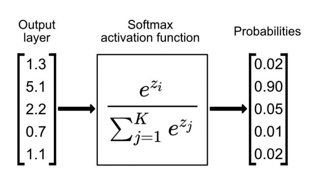
The process involves two main steps:

1. Exponentiation: We take the mathematical constant $e$ (approximately 2.718) and raise it to the power of each logit. This makes all values positive and has the nice effect of making larger logits disproportionately larger. For a logit $z_i$, we calculate $e^{z_i}$.
2. Normalization: We sum up all the exponentiated values from step 1. Then, we divide each individual exponentiated value by this sum. This scales everything down so that the final values are all between 0 and 1 and collectively sum to 1.

The formula for the softmax function applied to a single logit $z_i$ from a vector of logits z is:

Here, $K$ is the total number of classes.

Let's see this in action with a clear, animated example.

As the video highlights, the output of the softmax function gives us a set of values that:

• Are all between 0 and 1.
• Sum to 1.
• Preserve the original ranking of the logits.

This allows us to interpret the output as the model's predicted probability for each class.

Softmax in Practice with PyTorch

Given your experience with PyTorch, it's crucial to understand how softmax is used in a typical training and inference workflow. You might assume you should add a softmax layer to the end of your model definition, but the standard practice in PyTorch is a bit more nuanced.

For a clear explanation of the implementation details, please read the following resource.

To summarize the key practical point from the article:

• During training, you should design your model to output raw logits. The nn.CrossEntropyLoss function, which is the standard for multi-class classification, is optimized to take these raw logits as input. It performs a numerically stable version of log-softmax and the loss calculation internally.
• During inference (when you want to make predictions on new data), you take the model's logit output and manually apply the softmax function to get the interpretable probabilities.

Here's a quick code snippet illustrating this common pattern:

import torch
import torch.nn.functional as F




# Assume 'model' is your trained network and 'input_image' is a new image tensor




# 1. Get raw logits from the model during inference
model.eval() # Set the model to evaluation mode
with torch.no_grad():
    logits = model(input_image) # Shape: [batch_size, num_classes]




# 2. Convert logits to probabilities using the functional softmax
probabilities = F.softmax(logits, dim=1)




# 3. Get the predicted class by finding the index of the max probability
predicted_class = torch.argmax(probabilities, dim=1)

print(f"Logits: {logits}")
print(f"Probabilities: {probabilities}")
print(f"Predicted class index: {predicted_class}")

Conclusion

In this lesson, we bridged the gap between a network's raw output and a meaningful, probabilistic prediction. You've learned how the softmax function is the key component for multiclass classification models.

Key Takeaways:

• Neural networks for classification output raw scores called logits.
• The softmax function transforms these logits into a probability distribution by exponentiating each logit and normalizing by the sum of all exponentiated logits.
• The resulting probabilities are all between 0 and 1, sum to 1, and can be interpreted as the model's confidence in each class.
• In PyTorch, the standard practice is to let the model output raw logits and use nn.CrossEntropyLoss during training, which applies a stable log-softmax internally. For inference, you apply torch.nn.functional.softmax() to the logits to get probabilities.

Preview of the Next Lesson

We have now completed a full forward pass: from an input image, through linear and ReLU layers, to a final set of logits that we can turn into probabilities and compare against the true label to calculate a loss. But how does the network use this loss to learn? In the next lesson, we will intuitively explore backpropagation, the fundamental algorithm that allows the network to adjust its internal weights based on its mistakes.