Building an Image Classifier with PyTorch

Introduction

In our last session, we outlined the standard PyTorch training loop—the engine that drives model learning. You learned the four core steps: the forward pass, loss calculation, backward pass, and optimizer step. We saw this as a cycle that repeats over many epochs and batches.

Today, we're going to zoom in on the model component of that loop. The main goal of this lesson is to learn how to construct a multi-layer feedforward neural network in PyTorch for an image classification task. We'll focus on defining the network's architecture using PyTorch's nn.Module, preparing it to be dropped into the training loop we've already learned.

By the end of this 30-minute lesson, you will know how to build the Python class for a neural network, define its layers, and specify how data flows through it.

What is a Multi-Layer Feedforward Network?

A feedforward neural network is a model that processes information in one direction—from input to output. It's composed of layers of interconnected "neurons." A "multi-layer" network simply means it has one or more hidden layers between the input and output layers.

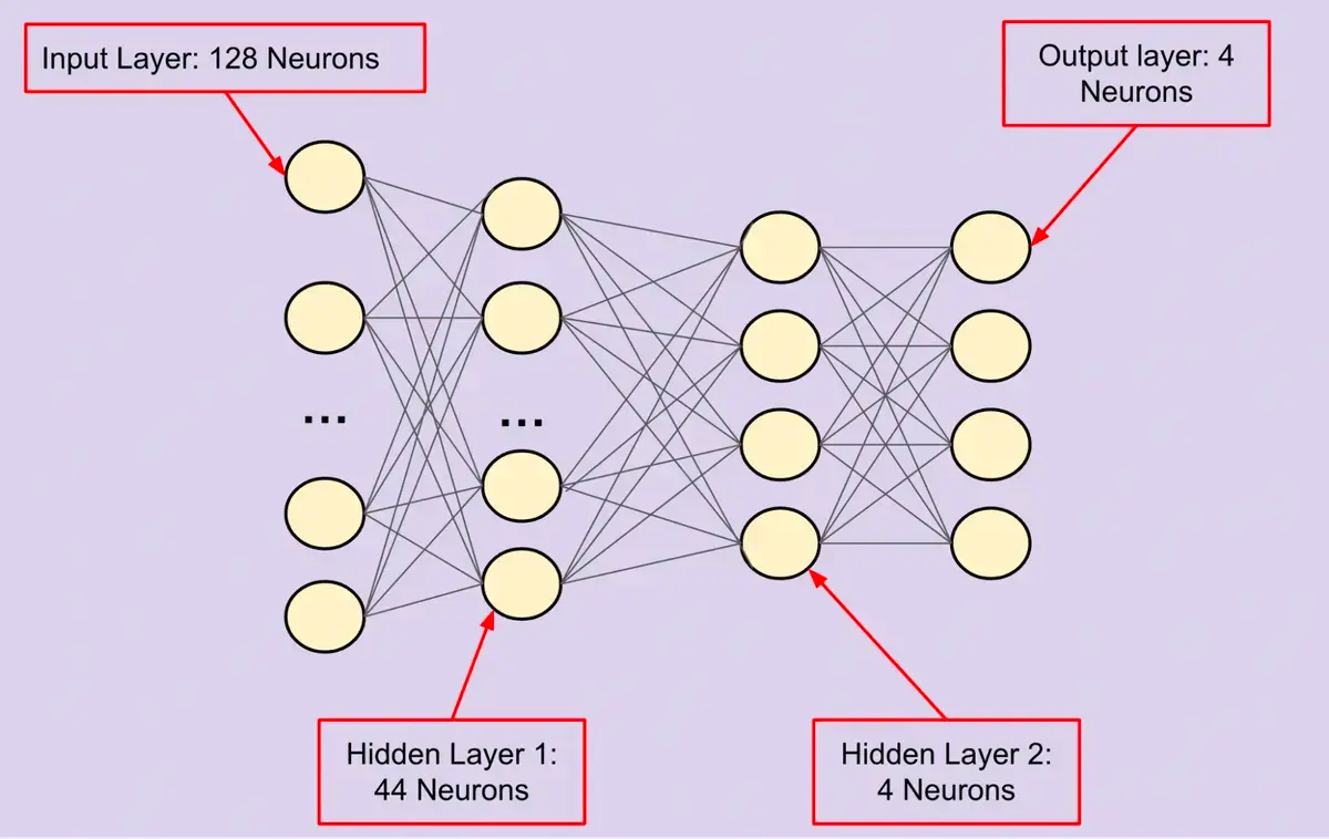
For an image classification task like recognizing handwritten digits (0-9), the architecture might look like this:

• Input Layer: Takes the flattened image pixels as input (e.g., a 28x28 image becomes a vector of 784 values).
• Hidden Layers: One or more layers that learn to recognize patterns and features from the input. These are the core of the network's learning capacity.
• Output Layer: Produces a score for each possible class (e.g., 10 scores, one for each digit).

These layers are typically "fully connected" (or Linear in PyTorch), meaning every neuron in one layer is connected to every neuron in the next.

The PyTorch Blueprint: nn.Module

In PyTorch, every neural network you build is a Python class that inherits from torch.nn.Module. This provides a standard "blueprint" with two essential methods you must define:

1. __init__(self): The constructor. Here, you define and initialize the layers of your network (e.g., linear layers, activation functions). Think of this as gathering your building materials.
2. forward(self, x): The forward pass. Here, you define the sequence of operations, specifying how the input data x flows through the layers you defined in __init__. This is like the assembly instruction manual.

Let's see this blueprint in action.

Constructing a Multi-Layer Network

As you saw in the video, we build the network by defining the layers in __init__ and connecting them in forward. Let's break down the code for a network with one hidden layer.

import torch
import torch.nn as nn




# Define hyperparameters
input_size = 784  # 28x28 pixels flattened
hidden_size = 100 # An arbitrary choice for the number of neurons in the hidden layer
num_classes = 10  # Digits 0-9

class NeuralNet(nn.Module):
    def __init__(self, input_size, hidden_size, num_classes):
        super(NeuralNet, self).__init__()



        # Define the layers
        self.fc1 = nn.Linear(input_size, hidden_size)  # First fully connected layer
        self.relu = nn.ReLU()                          # Non-linear activation (more on this next lesson!)
        self.fc2 = nn.Linear(hidden_size, num_classes) # Second fully connected layer (output)

    def forward(self, x):



        # Define the data flow
        out = self.fc1(x)
        out = self.relu(out)
        out = self.fc2(out)
        return out




# Instantiate the model
model = NeuralNet(input_size, hidden_size, num_classes)
print(model)

When you run this, you'll see a summary of the architecture PyTorch has built based on your class definition.

Notice the nn.ReLU() line. This is a non-linear activation function. Stacking only nn.Linear layers is mathematically equivalent to a single linear layer, which limits the model's power. Non-linearities are the key to learning complex patterns. We will dedicate our next lesson to understanding exactly what they do. For today, just know that we place them between our linear layers.

Building Deeper: A Two-Hidden-Layer Network

To make the network "multi-layer" in the truest sense, we can add more hidden layers. This is as simple as adding more nn.Linear and nn.ReLU layers in __init__ and adding them to the sequence in the forward method.

The pattern is clear:

1. Define a stack of alternating nn.Linear and nn.ReLU layers in __init__.
2. Pass the data through them sequentially in the forward method.

The input_dim of each layer must match the output_dim of the previous one, creating a chain.

Preparing the Data

Before we can feed an image into our network, we need to prepare it. Our network's first layer expects a 1D tensor of size 784, but the MNIST dataset provides 2D images of 28x28. We also need to load the data in batches. PyTorch's torchvision and DataLoader utilities make this easy.

Conclusion

In this lesson, you've learned the fundamental pattern for constructing neural network architectures in PyTorch. You now have the skills to build the model that fits into the training loop we discussed previously.

Key Takeaways:

• Neural networks in PyTorch are created by defining a class that inherits from nn.Module.
• The network's layers (e.g., nn.Linear) are defined in the __init__ method.
• The forward method defines the data's path through the network layers.
• Building a multi-layer network involves stacking linear layers, with non-linear activations placed in between.
• Image data must be flattened into a vector to be processed by a simple feedforward network's linear layers.

Preview of the Next Lesson

We've built the skeleton of a network, but we've glossed over two critical details. In the next lesson, we will dive into:

1. Non-linear Activation Functions: What is nn.ReLU() actually doing, and why is it essential for learning complex patterns?
2. Output Probabilities: How do we convert the raw output scores from our final layer into meaningful class probabilities using the softmax function?