PyTorch Multiclass Image Classification

Introduction

In our previous lessons, we've assembled all the individual components of a neural network training process. We learned how to:

1. Define a model architecture (nn.Module).
2. Perform a forward pass to get predictions.
3. Calculate the loss (nn.CrossEntropyLoss) to see how wrong the predictions are.
4. Perform a backward pass (loss.backward()) using backpropagation to calculate gradients.
5. Use an optimizer (optimizer.step()) to update the model's weights based on those gradients.

Today, we bring it all together. Our goal is to train a complete multiclass classification model from scratch using the full PyTorch training loop. We will use the famous MNIST dataset of handwritten digits, which is a classic "hello world" for image classification. By the end of this lesson, you will have trained a neural network that can look at an image of a handwritten digit and predict what number it is.

This is the capstone lesson for this module, where theory meets practice to create a working AI model.

1. Preparing the Data

Before we can train a model, we need data. PyTorch's torchvision library makes it incredibly easy to access standard datasets like MNIST. The two key classes we'll use are Dataset and DataLoader.

• Dataset: An object that stores the samples and their corresponding labels. For MNIST, this will be 60,000 training images and 10,000 testing images.
• DataLoader: An iterator that wraps a Dataset. It provides batches of data, shuffles the data every epoch, and can even use multiple subprocesses to load data in parallel. Training on small batches is more memory-efficient and can lead to better generalization than training on the whole dataset at once.

The following video provides a great walkthrough of setting up the MNIST dataset and creating DataLoaders.

Based on the video, here's the standard, simplified code to set up our data. Notice we only apply transforms.ToTensor(), which converts the images into PyTorch tensors.

import torch
from torch import nn
from torchvision import datasets, transforms
from torch.utils.data import DataLoader




# Define a transform to convert images to tensors
transform = transforms.ToTensor()




# Download and load the training data
train_data = datasets.MNIST(
    root="data",    # where to download
    train=True,     # get the training portion
    download=True,  # download if not on disk
    transform=transform
)




# Download and load the test data
test_data = datasets.MNIST(
    root="data",
    train=False,    # get the testing portion
    download=True,
    transform=transform
)




# Create DataLoaders
BATCH_SIZE = 32

train_dataloader = DataLoader(train_data, batch_size=BATCH_SIZE, shuffle=True)
test_dataloader = DataLoader(test_data, batch_size=BATCH_SIZE, shuffle=False)

print(f"DataLoaders created. {len(train_dataloader)} training batches of size {BATCH_SIZE}.")
print(f"Image batch shape: {next(iter(train_dataloader))[0].shape}")
print(f"Label batch shape: {next(iter(train_dataloader))[1].shape}")

You'll see that each batch of images has the shape [32, 1, 28, 28], which corresponds to [batch_size, color_channels, height, width].

2. Building the Neural Network

Now, let's define our model architecture. We will create a simple feedforward neural network. Since our nn.Linear layers expect a 1D vector of features for each sample, but our images are 2D (28x28), the first thing our model must do is flatten the image.

Here is the model definition. It subclasses nn.Module and defines the layers in __init__ and the forward pass logic in forward.

class MNISTClassifier(nn.Module):
    def __init__(self, input_shape: int, hidden_units: int, output_shape: int):
        super().__init__()
        self.layer_stack = nn.Sequential(
            nn.Flatten(), # Flattens the 28x28 image into a 784-element vector
            nn.Linear(in_features=input_shape, out_features=hidden_units),
            nn.ReLU(),
            nn.Linear(in_features=hidden_units, out_features=output_shape)
        )

    def forward(self, x: torch.Tensor):
        return self.layer_stack(x)




# Instantiate the model
model = MNISTClassifier(
    input_shape=784,  # 28*28
    hidden_units=128, # A common choice for a hidden layer size
    output_shape=10   # One output for each digit class (0-9)
)

print(model)

This model takes a batch of images, flattens each one, passes it through a hidden layer with a ReLU activation, and finally through an output layer that produces 10 raw scores (logits) for each image.

3. The Training Loop

This is where everything comes together. A training loop iterates over the dataset for a specified number of epochs. In each epoch, it iterates through every batch in the DataLoader. For each batch, it performs the full cycle: forward pass, loss calculation, backward pass, and optimizer step.

The diagram below provides a great visual summary of the process.

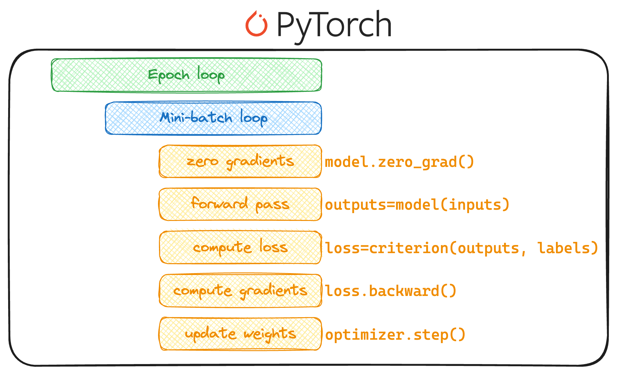
Now, let's write the code for this loop. We'll define our loss function (CrossEntropyLoss for multiclass classification) and our optimizer (SGD or Adam are good choices).

Here is a complete, runnable script that defines the model, sets up the loss and optimizer, and runs the training loop for a few epochs.

# Setup loss function and optimizer
loss_fn = nn.CrossEntropyLoss()
optimizer = torch.optim.Adam(params=model.parameters(), lr=0.001)




# --- Training Loop ---
epochs = 3
for epoch in range(epochs):
    print(f"Epoch: {epoch}\n---------")
    train_loss = 0



    # Put model in training mode
    model.train()
    
    for batch, (X, y) in enumerate(train_dataloader):



        # 1. Forward pass
        y_pred_logits = model(X)




        # 2. Calculate loss
        loss = loss_fn(y_pred_logits, y)
        train_loss += loss.item() # Use .item() to get the raw number




        # 3. Optimizer zero grad
        optimizer.zero_grad()




        # 4. Loss backward (backpropagation)
        loss.backward()




        # 5. Optimizer step (gradient descent)
        optimizer.step()




    # Calculate average training loss per batch
    train_loss /= len(train_dataloader)
    print(f"Average training loss: {train_loss:.5f}")

print("\nTraining complete!")

When you run this code, you should see the average training loss decrease with each epoch. This is a sign that your model is learning!

4. Evaluating the Model

A decreasing training loss shows the model is learning the training data, but it doesn't tell us if it can generalize to new, unseen data. To do that, we must evaluate it on our test_dataloader.

The evaluation loop is similar to the training loop, but with two key differences:

1. model.eval(): We put the model in "evaluation mode". This disables layers like Dropout or BatchNorm if they were present.
2. with torch.no_grad(): We wrap the loop in this context manager. It tells PyTorch not to calculate gradients, which saves memory and computation since we are not training.

# --- Evaluation Loop ---
test_loss = 0
test_acc = 0




# Put model in evaluation mode
model.eval()

with torch.no_grad():
    for X, y in test_dataloader:



        # 1. Forward pass
        test_pred_logits = model(X)




        # 2. Calculate loss
        test_loss += loss_fn(test_pred_logits, y).item()
        



        # 3. Calculate accuracy
        # Convert logits to prediction labels
        y_pred_labels = test_pred_logits.argmax(dim=1)
        test_acc += (y_pred_labels == y).sum().item() / len(y_pred_labels)




# Calculate average loss and accuracy over all batches
test_loss /= len(test_dataloader)
test_acc /= len(test_dataloader)

print(f"\nTest Results: \n  Accuracy: {(test_acc*100):.2f}% \n  Average loss: {test_loss:.5f}")

After only a few epochs, you should see an accuracy well above 90%. Congratulations, you've successfully trained a competent image classifier!

Conclusion

In this lesson, you integrated all the concepts from this module into a single, working application. You have mastered the fundamental PyTorch pipeline for supervised learning.

Key Takeaways:

• torchvision.datasets and DataLoader are essential tools for preparing and batching data for training.
• The training loop iterates through epochs and batches, performing the forward pass, loss calculation, backpropagation, and weight update cycle for each batch.
• The evaluation loop uses model.eval() and torch.no_grad() to efficiently measure model performance on unseen data without updating weights.
• You can now train a multiclass classification model for a standard image dataset like MNIST.

Preview of the Next Lesson

We've trained our model and calculated its overall accuracy. But what kind of mistakes is it making? Is it confusing 7s with 1s? Or 9s with 4s? In our final lesson of the course, we will dive deeper into model evaluation, learning how to use tools like a confusion matrix and class-specific metrics to get a much richer understanding of our model's performance.