Introduction
Hello! In our last lesson, we put the K-means algorithm into practice. You learned how to implement it using scikit-learn and how to use the elbow method to select a suitable number of clusters, K. This gave you a solid workflow for applying K-means to a dataset.
However, a crucial part of being an effective practitioner is knowing not just how to use a tool, but also understanding its limitations. This lesson focuses on exactly that. Our goal is to identify the limitations of K-means, such as its sensitivity to initial centroids and its difficulty with non-convex clusters. Understanding these weaknesses will help you diagnose problems and know when a different clustering algorithm might be a better choice.
Limitation 1: Sensitivity to Initial Centroids
The K-means algorithm you learned about—assigning points and updating centroids—has a critical dependency: its final result can change based on the initial placement of the centroids. If the centroids start in "unlucky" positions, the algorithm can converge to a suboptimal solution (a local minimum) that doesn't represent the best possible clustering.
The following short video provides a clear, interactive demonstration of this exact problem.
Watch this video from Orange Data Mining to see how different starting positions for the centroids lead to completely different final clusters, even on the same data.
Please watch from 00:45 to 01:41. The presenter manually places centroids in different starting locations and runs the K-means algorithm, showing how a poor initialization leads to an incorrect clustering.
As you saw, a bad random start can cause K-means to split a natural cluster or incorrectly merge distinct ones. So, how do we address this?
The Solution: K-means++
Fortunately, this problem has a well-established solution called K-means++. Instead of placing centroids completely at random, K-means++ uses a smarter initialization technique. It places the first centroid randomly, but then chooses subsequent centroids from the data points with a probability proportional to their distance from the nearest existing centroid. This strategy favors spreading out the initial centroids, making it much more likely that the algorithm will converge to a good solution.
The good news is that you are already using it! Modern libraries like scikit-learn use the K-means++ initialization by default.
# The default initialization is 'k-means++'
# You've been using it all along!
kmeans = KMeans(n_clusters=3, init='k-means++', n_init=10, random_state=42)
The parameter n_init=10 is also important. It tells scikit-learn to run the entire K-means algorithm 10 times with different K-means++ initializations and return the best result (the one with the lowest inertia). This makes the algorithm far more robust to the problem of random starting points.
Limitation 2: The Spherical Cluster Assumption
K-means identifies clusters based on a single, simple rule: assigning each point to the nearest centroid. This use of Euclidean distance inherently assumes that clusters are convex and isotropic—meaning they are roughly spherical and have a similar radius.
When clusters are elongated, have irregular shapes, or are intertwined, K-means often fails to identify them correctly.
K-Means Advantages and Disadvantages
This clip from TheDataPost demonstrates how K-means fails on a simple non-convex dataset.
Watch from 01:07 to 01:41. You'll see K-means attempt to cluster a 'smiley face' dataset, where it incorrectly partitions the data into quadrants instead of identifying the eyes and mouth as separate clusters.
This limitation isn't just for smiley faces. It applies to any dataset where the underlying groups aren't blob-like. The image below, from the scikit-learn documentation, showcases several scenarios where K-means produces counter-intuitive results because its assumptions about the data shape are violated.
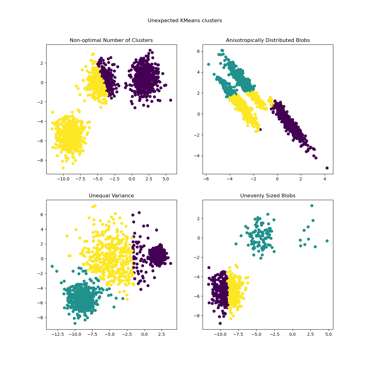
Because K-means only cares about the distance to a central point, it is fundamentally incapable of capturing the more complex structure seen in these examples.
The following image provides one final, powerful comparison. It shows K-means failing on intertwined, non-convex clusters, and contrasts it with the output of another algorithm.
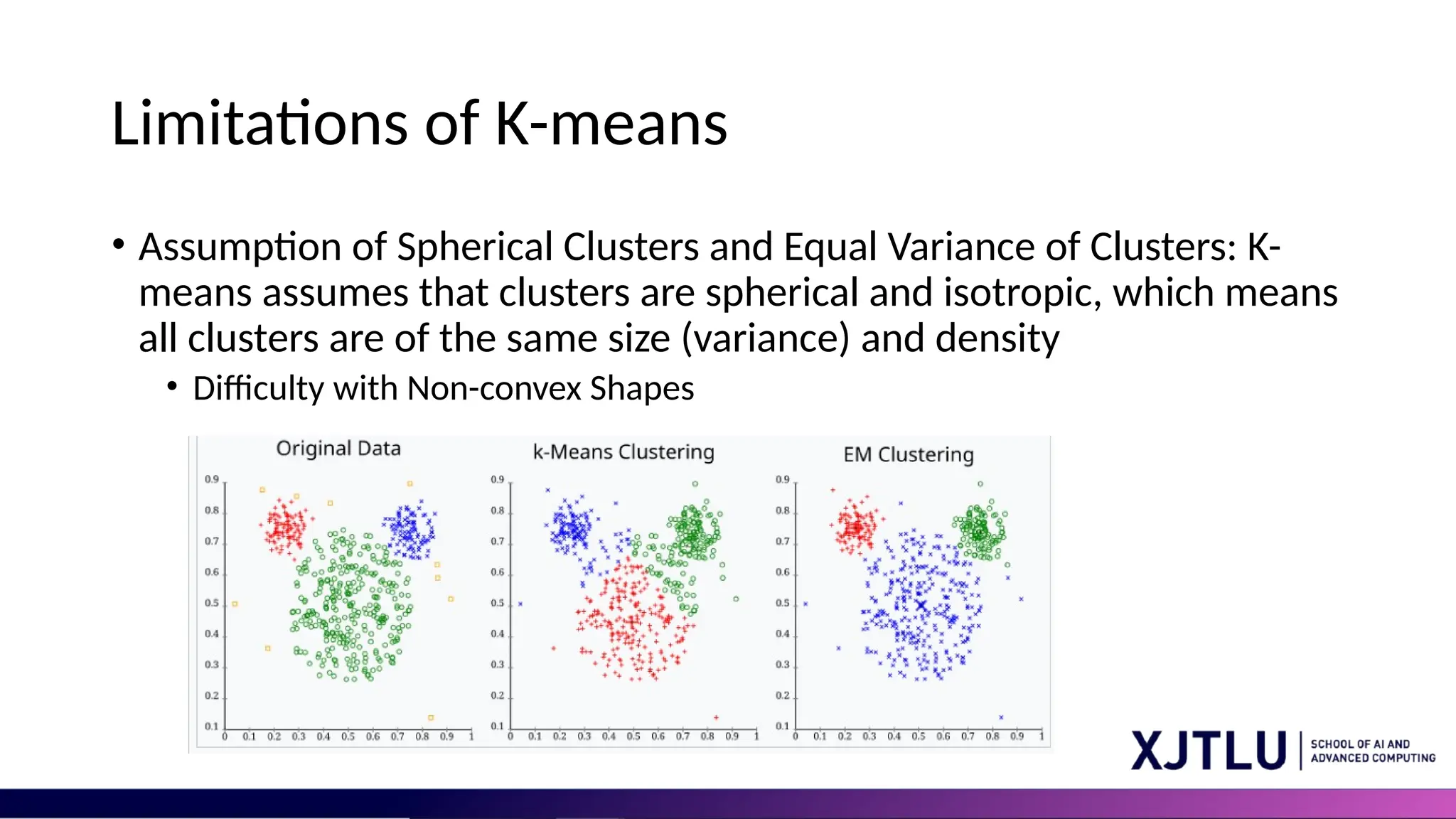
The algorithm on the right, EM (Expectation-Maximization), is what powers Gaussian Mixture Models, the topic of our next lesson. It represents a move away from the "hard" assignments of K-means to a more flexible, probabilistic approach that can handle these complex shapes.
Conclusion
In this lesson, we explored the critical limitations of the K-means algorithm. While powerful and efficient, its effectiveness depends on the structure of your data.
Key Takeaways:
- Sensitivity to Initialization: The standard K-means algorithm can produce different results based on where the centroids start. This is mitigated in practice by using the K-means++ initialization method and running the algorithm multiple times (
n_init), which are the defaults inscikit-learn. - Difficulty with Non-Convex Clusters: K-means assumes clusters are spherical and evenly sized because it relies on distance to a central point. It performs poorly on datasets with elongated, irregular, or intertwined clusters.
- Understanding these limitations is key to interpreting K-means results and knowing when to choose a more suitable algorithm.
Preview of the Next Lesson
You've just seen a preview of where we're headed. The K-means algorithm performs what is known as "hard clustering," where every point belongs to exactly one cluster. To overcome its limitations with cluster shapes, we need a more flexible approach. In the next lesson, we will explore Gaussian Mixture Models (GMMs), which perform "soft" or probabilistic clustering, allowing them to model a much wider variety of cluster shapes.